Complex numbers and quaternions

(ns complex-quaternions
  (:require [fastmath.complex :as cplx]
            [fastmath.quaternion :as quat]
            [fastmath.vector :as v]
            [fastmath.dev.codox :as codox]
            [fastmath.dev.ggplot :as gg]
            [fastmath.dev.clay :as utls]
            [scicloj.kindly.v4.kind :as kind]
            [fastmath.core :as m]
            [fastmath.matrix :as mat]))

Complex numbers

Defined functions

complex, ensure-complex

Complex numbers extend the concept of real numbers by including an imaginary unit $i$, where $i^2 = -1$.

In fastmath, complex numbers are represented as 2-dimensional vectors using the fastmath.vector/Vec2 type, where the x-component is the real part and the y-component is the imaginary part.

You can create complex numbers using the dedicated complex function, the general 2D vector constructor fastmath.vector/vec2, or by converting sequences/arrays using functions like fastmath.vector/seq->vec2. ensure-complex accepts single argument which can be a real or complex number.

Examples

(cplx/complex) ;; => #vec2 [0.0, 0.0]
(cplx/complex 1.0) ;; => #vec2 [1.0, 0.0]
(cplx/complex 1.0 -2.0) ;; => #vec2 [1.0, -2.0]
(v/vec2 1.0 -2.0) ;; => #vec2 [1.0, -2.0]
(v/seq->vec2 [1.0 -2.0]) ;; => #vec2 [1.0, -2.0]
(cplx/ensure-complex 2.0) ;; => #vec2 [2.0, 0.0]
(cplx/ensure-complex (cplx/complex 1.0 -2.0)) ;; => #vec2 [1.0, -2.0]

The implementation handles floating-point subtleties, including special values (##Inf, ##NaN) and signed zero (+0.0, -0.0), for robust calculations across a wide range of inputs.

This section covers constants, predicates, and a comprehensive set of operations including basic arithmetic, exponentiation, logarithms, trigonometric functions, and their inverses.

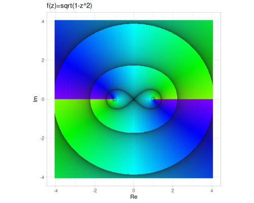
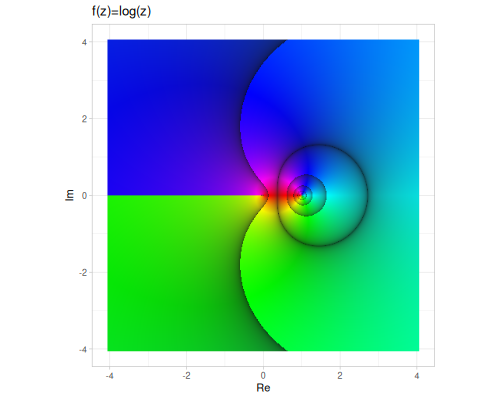
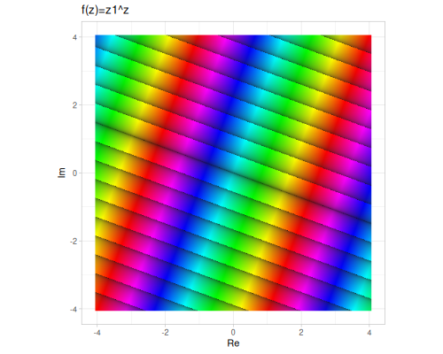
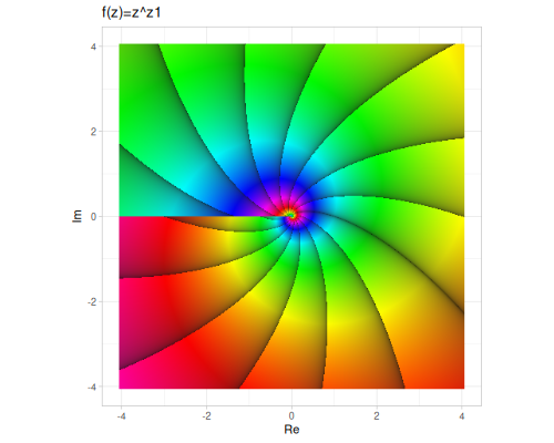
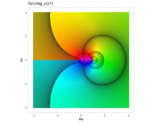
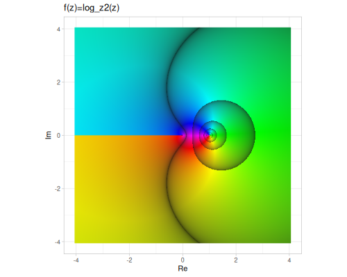
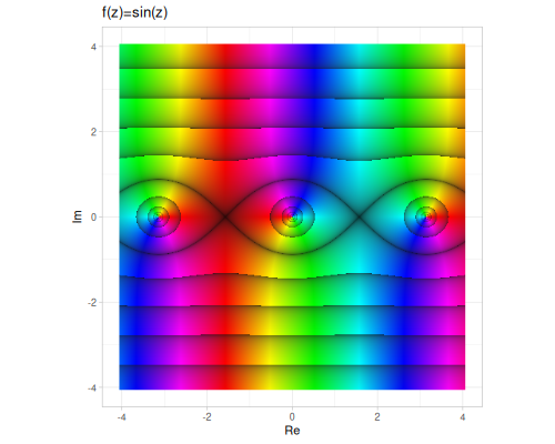
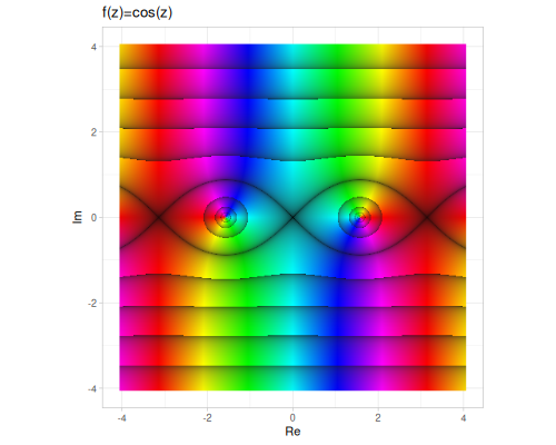
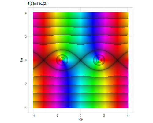
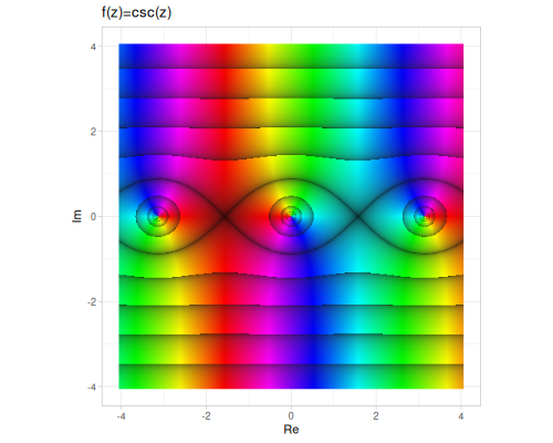
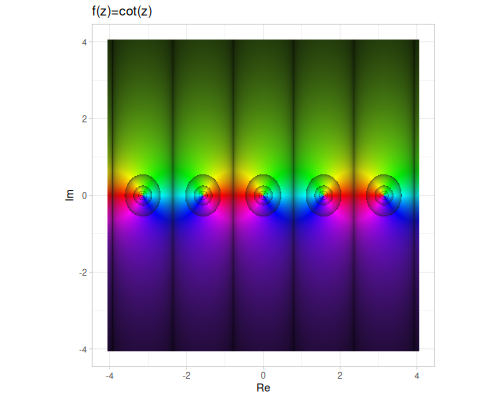
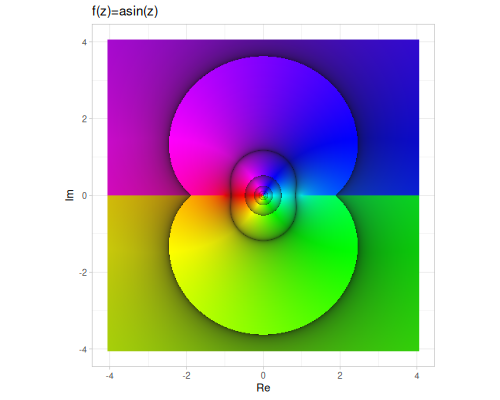
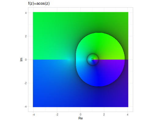
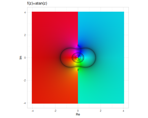
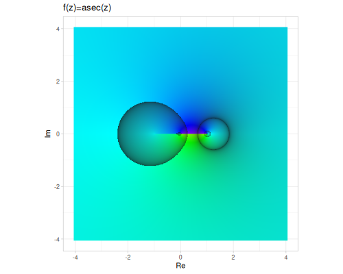
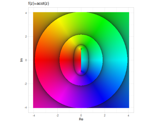
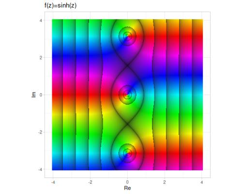
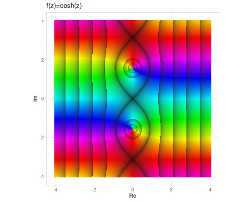
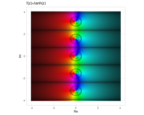
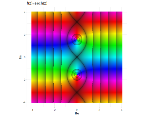
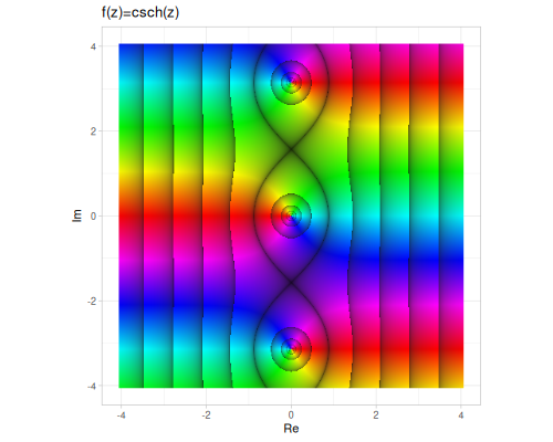
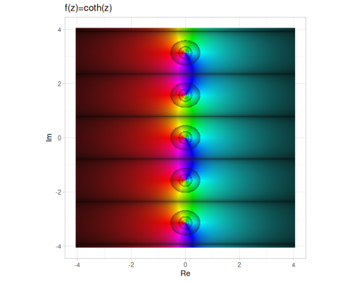
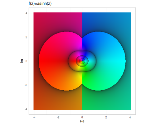
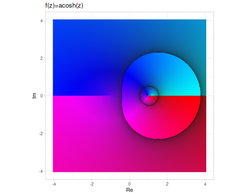
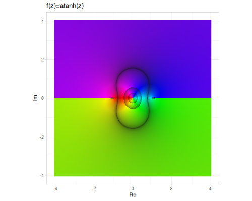
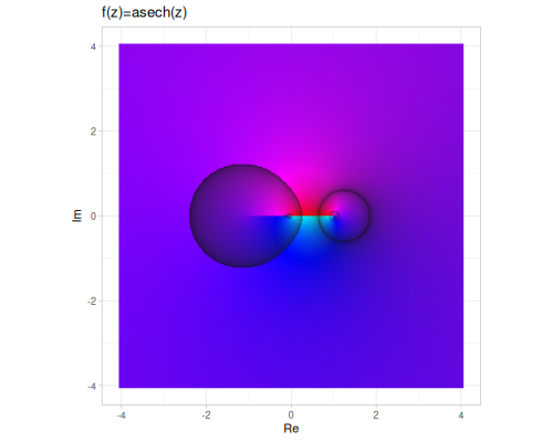
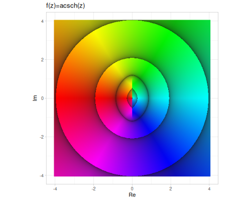
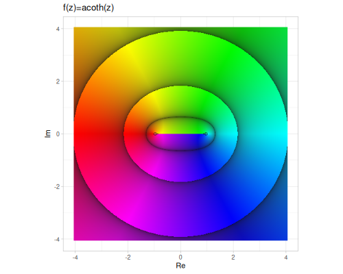
Plots are based on domain coloring in HSB space, where

hue - represents argument
saturation/brightness - represents fractional part of logarithm of magnitude

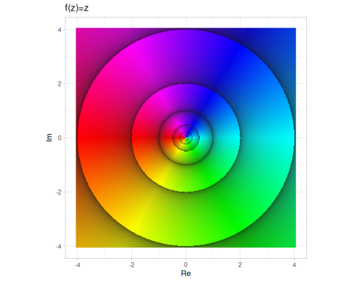
We will use these numbers to illustrate operations:

(def z1 (cplx/complex 0.5 -1.5))

(def z2 (cplx/complex -0.5 2.5))

(def z3 (cplx/complex 1.5 0.5))

Examples

z1 ;; => #vec2 [0.5, -1.5]
z2 ;; => #vec2 [-0.5, 2.5]
z3 ;; => #vec2 [1.5, 0.5]

Constants

List of defined complex constants.

constant	z	value
I	$0+i$	#vec2 [0.0, 1.0]
-I	$0-i$	#vec2 [0.0, -1.0]
I-	$0-i$	#vec2 [0.0, -1.0]
ZERO	$0+0i$	#vec2 [0.0, 0.0]
ONE	$1+0i$	#vec2 [1.0, 0.0]
TWO	$2+0i$	#vec2 [2.0, 0.0]
PI	$\pi+0i$	#vec2 [3.141592653589793, 0.0]

Basic operations

This section provides a collection of functions for performing fundamental operations on complex numbers. These operations include extracting components, calculating magnitude and argument, finding conjugates, performing arithmetic (addition, subtraction, multiplication, division), negation, reciprocals, and square roots.

Defined functions

re, im
delta-eq, csgn, flip
abs, norm, normalize, conjugate
arg
add, adds, sub, neg
scale, mult, mult-I, mult-I-, muladd, sq
div, reciprocal
sqrt, sqrt1z

Components
- re: Returns the real part of a complex number $z$. For $z = a + bi$, returns $a$.
- im: Returns the imaginary part of a complex number $z$. For $z = a + bi$, returns $b$.

Examples

(cplx/re z1) ;; => 0.5
(cplx/im z1) ;; => -1.5

Properties and Comparisons
- abs: Calculates the magnitude or modulus of a complex number $|z|$. For $z = a + bi$: \[|z| = \sqrt{a^2 + b^2}\] This corresponds to the length of the vector (Vec2. a b).
- norm: Calculates the squared magnitude $|z|^2$. For $z = a + bi$: \[|z|^2 = a^2 + b^2\] This avoids the square root calculation and is often used when comparing magnitudes.
- arg: Computes the argument (phase angle) of a complex number $z$. This is the angle $\phi$ such that $z = |z| (\cos \phi + i \sin \phi)$, and is typically in the range $(-\pi, \pi]$. Calculated as: \[\operatorname{arg}(z)=\operatorname{atan2}(\operatorname{im}(z), \operatorname{re}(z))\]
- normalize: Sets magnitude of a complex number $z$ to 1.0: \[\frac{z}{|z|}\]
- conjugate: Returns the complex conjugate of $z$, denoted $\bar{z}$. For $z = a + bi$: \[\bar{z} = a - bi\] Geometrically, this is a reflection across the real axis.
- flip: Swaps the real and imaginary parts of a complex number. For $z = a + bi$, returns $b + ai$.
- delta-eq: Checks if two complex numbers are approximately equal within a given tolerance. This is essential for floating-point comparisons and equivalent to checking if $|z_1 - z_2| < \text{tolerance}$.
- csgn: Implements the complex signum function. Returns 0 for the zero complex number. For non-zero $z$, it returns the sign of the real part $\operatorname{sgn}(\operatorname{re}(z))$.

Examples

z1 ;; => #vec2 [0.5, -1.5]
(cplx/abs z1) ;; => 1.5811388300841898
(cplx/norm z1) ;; => 2.5
(cplx/arg z1) ;; => -1.2490457723982544
(cplx/normalize z1) ;; => #vec2 [0.31622776601683794, -0.9486832980505138]
(cplx/abs (cplx/normalize z1)) ;; => 0.9999999999999999
(cplx/conjugate z1) ;; => #vec2 [0.5, 1.5]
(cplx/flip z1) ;; => #vec2 [-1.5, 0.5]
z2 ;; => #vec2 [-0.5, 2.5]
(cplx/abs z2) ;; => 2.5495097567963922
(cplx/norm z2) ;; => 6.5
(cplx/arg z2) ;; => 1.7681918866447774
(cplx/normalize z2) ;; => #vec2 [-0.19611613513818404, 0.9805806756909202]
(cplx/abs (cplx/normalize z2)) ;; => 1.0
(cplx/conjugate z2) ;; => #vec2 [-0.5, -2.5]
(cplx/flip z2) ;; => #vec2 [2.5, -0.5]
(cplx/csgn z1) ;; => 1.0
(cplx/csgn z2) ;; => -1.0
(cplx/csgn cplx/ZERO) ;; => 0.0
(cplx/delta-eq (cplx/complex 0.001) cplx/ZERO) ;; => false
(cplx/delta-eq (cplx/complex 0.001) cplx/ZERO 0.01) ;; => true

Arithmetic Operations
- add: Computes the sum of two complex numbers, $z_1 + z_2$. If $z_1 = a + bi$ and $z_2 = c + di$: \[z_1 + z_2 = (a+c) + (b+d)i\]
- adds: Adds a real scalar $s$ to a complex number $z$. For $z = a + bi$: \[z + s = (a+s) + bi\]
- sub: Computes the difference of two complex numbers, $z_1 - z_2$. If $z_1 = a + bi$ and $z_2 = c + di$: \[z_1 - z_2 = (a-c) + (b-d)i\]
- neg: Returns the negation of a complex number, $-z$. For $z = a + bi$: \[-z = -a - bi\]
- scale: Multiplies a complex number $z$ by a real scalar $s$. For $z = a + bi$: \[z \cdot s = (as) + (bs)i\]
- mult: Computes the product of two complex numbers, $z_1 \cdot z_2$. If $z_1 = a + bi$ and $z_2 = c + di$: \[z_1 \cdot z_2 = (ac - bd) + (ad + bc)i\]
- mult-I: Multiplies a complex number $z$ by the imaginary unit $i$. For $z = a + bi$: \[z \cdot i = -b + ai\]
- mult-I-: Multiplies a complex number $z$ by $-i$. For $z = a + bi$: \[z \cdot (-i) = b - ai\]
- muladd: Computes the fused multiply-add operation \[(x \cdot y) + z\] for complex numbers $x, y, z$.
- sq: Computes the square of a complex number, $z^2$. For $z = a + bi$: \[z^2 = (a^2 - b^2) + 2abi\]
- div: Computes the division of two complex numbers, $z_1 / z_2$. If $z_1 = a + bi$ and $z_2 = c + di$: \[z_1 / z_2 = \frac{z_1 \cdot \bar{z_2}}{|z_2|^2} = \frac{(ac+bd) + (bc-ad)i}{c^2+d^2}\]
- reciprocal: Computes the reciprocal of a complex number, $1/z$. For $z = a + bi$: \[1/z = \frac{\bar{z}}{|z|^2} = \frac{a - bi}{a^2+b^2}\]

Examples

(cplx/add z1 z2) ;; => #vec2 [0.0, 1.0]
(cplx/adds z1 -3.5) ;; => #vec2 [-3.0, -1.5]
(cplx/sub z1 z2) ;; => #vec2 [1.0, -4.0]
(cplx/neg z1) ;; => #vec2 [-0.5, 1.5]
(cplx/scale z1 5) ;; => #vec2 [2.5, -7.5]
(cplx/mult z1 z2) ;; => #vec2 [3.5, 2.0]
(cplx/mult-I z1) ;; => #vec2 [1.5, 0.5]
(cplx/mult-I- z1) ;; => #vec2 [-1.5, -0.5]
(cplx/muladd z1 z2 z3) ;; => #vec2 [5.0, 2.5]
(cplx/sq z1) ;; => #vec2 [-2.0, -1.5]
(cplx/div z1 z2) ;; => #vec2 [-0.6153846153846154, -0.07692307692307693]
(cplx/reciprocal z1) ;; => #vec2 [0.2, 0.6]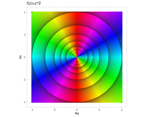

Roots
- sqrt: Computes the principal square root of a complex number: \[\sqrt{z} = \sqrt{\frac{|a| + x}{2}} + i \cdot \operatorname{sgn}(b) \cdot \sqrt{\frac{|z| - a}{2}}\]
- sqrt1z: Computes $\sqrt{1 - z^2}$ for a complex number $z$.

Examples

(cplx/sqrt z1) ;; => #vec2 [1.0200830432087846, -0.7352342586156434]
(cplx/sqrt z2) ;; => #vec2 [1.0123017723970438, 1.2348096526988264]
(cplx/sqrt z3) ;; => #vec2 [1.2411967672541269, 0.20141850719855633]
(cplx/sqrt1z z1) ;; => #vec2 [1.782428394950227, 0.4207742662340966]
(cplx/sqrt1z z2) ;; => #vec2 [2.686357605909836, 0.46531407331997443]
(cplx/sqrt1z z3) ;; => #vec2 [0.6335517491618166, -1.1838022718621541]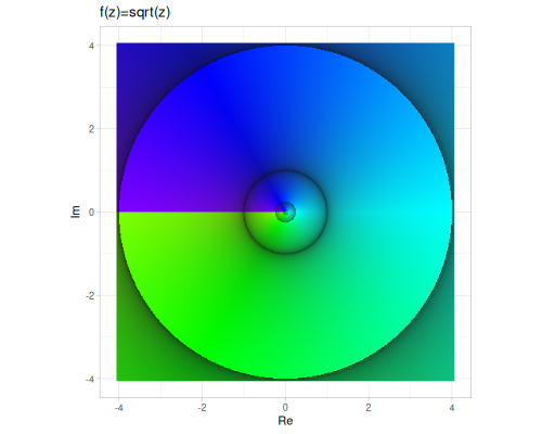

Predicates

Predicates are functions that return a boolean value, indicating whether a complex number satisfies a specific condition. They are useful for checking the nature or state of a complex number, such as whether it is real, imaginary, zero, infinite, or invalid.

Defined functions

real?, imaginary?
zero?
inf?,nan?
invalid?, valid?

real?: Checks if a complex number z has a zero imaginary part. $z = a + bi$ is real if $b = \operatorname{im}(z) = 0$.
imaginary?: Checks if a complex number z has a zero real part. $z = a + bi$ is pure imaginary if $a = \operatorname{re}(z) = 0$.
zero?: Checks if z is the complex number $0+0i$, which is true if both real and imaginary parts are zero.
inf?: Checks if either the real or imaginary part of z is positive or negative infinity (##Inf or ##-Inf).
nan?: Checks if either the real or imaginary part of z is Not a Number (##NaN).
invalid?: Checks if z is either inf? or nan?. Represents values that are not finite numbers.
valid?: Checks if z is a finite, non-NaN number. This is the opposite of invalid?.

Examples

(cplx/real? cplx/ONE) ;; => true
(cplx/real? cplx/I) ;; => false
(cplx/imaginary? cplx/ONE) ;; => false
(cplx/imaginary? cplx/I) ;; => true
(cplx/zero? cplx/ZERO) ;; => true
(cplx/zero? cplx/ONE) ;; => false
(cplx/inf? (cplx/complex ##Inf 1)) ;; => true
(cplx/nan? (cplx/complex 1 ##NaN)) ;; => true
(cplx/invalid? (cplx/complex ##Inf 1)) ;; => true
(cplx/invalid? (cplx/complex 1.0 2.0)) ;; => false
(cplx/valid? (cplx/complex 1.0 2.0)) ;; => true
(cplx/valid? (cplx/complex ##Inf 1)) ;; => false

Power and logarithms

Complex numbers extend the real-valued exponential and logarithm functions. Complex exponentiation allows raising a complex base to a complex power, while the complex logarithm is the inverse operation of exponentiation. Unlike real logarithms, the complex logarithm is multi-valued, but the functions provided here compute the principal value.

Defined functions

pow, exp
log, logb

exp: Computes the complex exponential $e^z$. For $z = x + iy$: \[e^z = e^{x+iy} = e^x (\cos y + i \sin y)\]
log: Computes the principal value of the complex natural logarithm $\log z$. This is given by: \[\log z = \ln|z| + i \arg(z)\] where $\ln|z|$ is the real natural logarithm of the magnitude $|z|$, and $\arg(z)$ is the principal argument of $z$.
logb: Computes the logarithm of $z$ with a complex base $b$: \[\log_b z = \frac{\log z}{\log b}\]
pow: Computes the complex power $z_1^{z_2}$. This is defined as \[z_1^{z_2} = e^{z_2 \log z_1}\] where $\log z_1$ is the principal value of the logarithm. Handles various edge cases, including $0^0$.

Examples

(cplx/exp z1) ;; => #vec2 [0.11662592901934625, -1.644591201830844]
(cplx/log z1) ;; => #vec2 [0.45814536593707755, -1.2490457723982544]
(cplx/logb z1 z2) ;; => #vec2 [-0.4446751692907921, -0.4944697164867257]
(cplx/pow z1 z2) ;; => #vec2 [-3.571295577918147, 17.700466856264484]
(cplx/pow z3 z1) ;; => #vec2 [1.761680541256831, -1.0235623709790516]
(cplx/pow cplx/ZERO cplx/ZERO) ;; => #vec2 [NaN, NaN]
(cplx/pow cplx/ZERO (cplx/complex 1 1)) ;; => #vec2 [0.0, 0.0]
(cplx/pow (cplx/complex 1 1) cplx/ZERO) ;; => #vec2 [1.0, 0.0]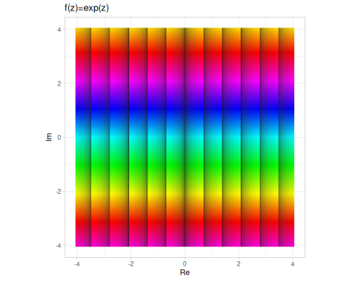

Trigonometric and Hyperbolic

Complex trigonometric and hyperbolic functions extend their real-valued counterparts to the complex plane. They are defined in terms of the complex exponential function:

\[ \sin z = \frac{e^{iz} - e^{-iz}}{2i} \quad \cos z = \frac{e^{iz} + e^{-iz}}{2} \] \[ \sinh z = \frac{e^{z} - e^{-z}}{2} \quad \cosh z = \frac{e^{z} + e^{-z}}{2} \]

This leads to relationships between complex trigonometric and hyperbolic functions, such as $\sin(z) = -i \sinh(iz)$ and $\cos(z) = \cosh(iz)$. These functions are implemented using formulas that provide numerical stability, especially for large arguments.

Defined functions

sin, cos, tan
sec, csc, cot
sinh, cosh, tanh
sech, csch, coth
asin, acos, atan
asec, acsc, acot
asinh, acosh, atanh
asech, acsch, acoth

Standard Trigonometric Functions: sin, cos, tan, sec, csc, cot
- These are the direct extensions of real trigonometric functions. For $z = x + iy$: \[ \sin z = \sin x \cosh y + i \cos x \sinh y \] \[ \cos z = \cos x \cosh y - i \sin x \sinh y \] \[ \tan z = \frac{\sin x \cos x + i \sinh y \cosh y}{\cos^2 x + \sinh^2 y} \]
- sec(z), csc(z), and cot(z) are computed as the reciprocals of cos(z), sin(z), and tan(z), respectively.
Hyperbolic Trigonometric Functions: sinh, cosh, tanh, sech, csch, coth
- These are also extensions of real hyperbolic functions. For $z = x + iy$: \[ \sinh z = \sinh x \cos y + i \cosh x \sin y \] \[ \cosh z = \cosh x \cos y + i \sinh x \sin y \] \[ \tanh z = \frac{\sinh x \cosh x + i \sin y \cos y}{\sinh^2 x + \cos^2 y} \]
- sech(z), csch(z), and coth(z) are computed as the reciprocals of cosh(z), sinh(z), and tanh(z), respectively.
Inverse Trigonometric Functions: asin, acos, atan, asec, acsc, acot
- These are the multi-valued inverse functions. The implementations return the principal values, which are related to complex logarithms. For example: \[ \arcsin z = -i \log(iz + \sqrt{1-z^2}) \] \[ \arccos z = -i \log(z + i\sqrt{1-z^2}) \] \[ \arctan z = \frac{i}{2} \log\left(\frac{1-iz}{1+iz}\right) \] \[ \operatorname{arcsec} z = \arccos(1/z) \] \[ \operatorname{arccsc} z = \arcsin(1/z) \] \[ \operatorname{arccot} z = \operatorname{atan}(1/z) \]
Inverse Hyperbolic Trigonometric Functions: asinh, acosh, atanh, asech, acsch, acoth
- These are the multi-valued inverse hyperbolic functions. The implementations return the principal values, which are also related to complex logarithms. For example: \[ \operatorname{arsinh} z = \log(z + \sqrt{z^2+1}) \] \[ \operatorname{arcosh} z = \log(z + \sqrt{z^2-1}) \] \[ \operatorname{artanh} z = \frac{1}{2} \log\left(\frac{1+z}{1-z}\right) \] \[ \operatorname{arsech} z = \operatorname{arcosh}(1/z) \] \[ \operatorname{arcsch} z = \operatorname{arsinh}(1/z) \] \[ \operatorname{arcoth} z = \operatorname{artanh}(1/z) \]

These functions are continuous and analytic everywhere in the complex plane, except at certain points (poles) where the denominator is zero for tangent, cotangent, secant, cosecant, and at branch cuts for the inverse functions.

Examples

(cplx/sin z1) ;; => #vec2 [1.1278052468056998, -1.868618519182647]
(cplx/cos z1) ;; => #vec2 [2.0644336567607153, 1.0208309495976968]
(cplx/tan z1) ;; => #vec2 [0.07932445480395665, -0.9443729864226214]
(cplx/sec z1) ;; => #vec2 [0.38922334164348615, -0.1924650047020439]
(cplx/csc z1) ;; => #vec2 [0.23675084882124306, 0.3922636659056108]
(cplx/cot z1) ;; => #vec2 [0.08832153001414375, 1.0514849080401338]
(cplx/asin z1) ;; => #vec2 [0.2734872901415567, -1.2264568712514057]
(cplx/acos z1) ;; => #vec2 [1.2973090366533397, 1.2264568712514057]
(cplx/atan z1) ;; => #vec2 [1.2767950250211129, -0.6412373393653842]
(cplx/asec z1) ;; => #vec2 [1.3991340865479363, -0.5764844975630772]
(cplx/acsc z1) ;; => #vec2 [0.17166224024696028, 0.5764844975630772]
(cplx/acot z1) ;; => #vec2 [0.2940013017737837, 0.6412373393653842]
(cplx/sinh z1) ;; => #vec2 [0.03686082371280443, -1.1248012470579227]
(cplx/cosh z1) ;; => #vec2 [0.07976510530654181, -0.5197899547729212]
(cplx/tanh z1) ;; => #vec2 [2.1247991277429965, -0.25514922181365146]
(cplx/sech z1) ;; => #vec2 [0.28843542211554024, 1.8795917643457205]
(cplx/csch z1) ;; => #vec2 [0.02910363957175099, 0.8880922016091114]
(cplx/coth z1) ;; => #vec2 [0.46394286018382835, 0.05571098848654149]
(cplx/asinh z1) ;; => #vec2 [1.0693110431581105, -1.1711572594583723]
(cplx/acosh z1) ;; => #vec2 [-1.2264568712514057, 1.2973090366533397]
(cplx/atanh z1) ;; => #vec2 [0.14694666622552977, -1.0172219678978514]
(cplx/asech z1) ;; => #vec2 [0.5764844975630772, 1.3991340865479363]
(cplx/acsch z1) ;; => #vec2 [0.24366128541928853, 0.6219473660246817]
(cplx/acoth z1) ;; => #vec2 [0.14694666622552977, 0.5535743588970452]

sin	cos	tan

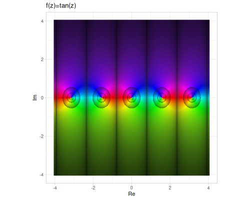sec	csc	cot

asin	acos	atan

asec	acsc	acot

sinh	cosh	tanh

sech	csch	coth

asinh	acosh	atanh

asech	acsch	acoth

Quaternions

Defined functions

quaternion, complex->quaternion, ensure-quaternion

Quaternions extend complex numbers with three imaginary units: $i$, $j$, and $k$, satisfying the relations $i^2 = j^2 = k^2 = ijk = -1$. They are particularly useful for representing 3D rotations concisely and avoiding gimbal lock.

In fastmath, quaternions are represented as 4-dimensional vectors using the fastmath.vector/Vec4 type. A quaternion $q = a + bi + cj + dk$ corresponds to the vector (Vec4. a b c d), where $a$ is the scalar (real) part, and $(b, c, d)$ is the vector (imaginary) part.

You can create quaternions using the dedicated quaternion function, or by converting numbers or complex numbers using ensure-quaternion.

The implementation handles floating-point subtleties, including special values (##Inf, ##NaN), for robust calculations across a wide range of inputs.

This section covers constants, creation, accessors, predicates, basic operations, and advanced functions including power, logarithms, trigonometric functions, and functions specific to 3D rotations.

Examples

(quat/quaternion 1.0 -2.0 3.0 -4.0) ;; => #vec4 [1.0, -2.0, 3.0, -4.0]
(quat/quaternion 5.0 [1.0 2.0 3.0]) ;; => #vec4 [5.0, 1.0, 2.0, 3.0]
(quat/quaternion 7.0) ;; => #vec4 [7.0, 0.0, 0.0, 0.0]
(quat/complex->quaternion (cplx/complex 1.0 -2.0)) ;; => #vec4 [1.0, -2.0, 0.0, 0.0]
(quat/ensure-quaternion 5.0) ;; => #vec4 [5.0, 0.0, 0.0, 0.0]
(quat/ensure-quaternion (cplx/complex 1.0 -2.0)) ;; => #vec4 [1.0, -2.0, 0.0, 0.0]

We will use these quaternions to illustrate operations:

(def q1 (quat/quaternion 0.5 -1.5 2.0 -0.5))

(def q2 (quat/quaternion -0.5 2.5 -1.0 1.5))

(def q3 (quat/quaternion 1.5 0.0 0.0 0.0))

(def q4 (quat/quaternion 0.0 1.0 -2.0 3.0))

Examples

q1 ;; => #vec4 [0.5, -1.5, 2.0, -0.5]
q2 ;; => #vec4 [-0.5, 2.5, -1.0, 1.5]
q3 ;; => #vec4 [1.5, 0.0, 0.0, 0.0]
q4 ;; => #vec4 [0.0, 1.0, -2.0, 3.0]

All of the trigonometric, hyperbolic, exp, log and sqrt functions are based on the following general formula. Let $r_q$ is the real part and $v_q$ is the vector (imaginary) part of quaternion $q$. Let $z_{in}$ is defined as follows:

\[z_{in} = r_q + |v_q|i\]

Then, if $f_z$ is given operation on complex number, corresponding quaternion version $f_q$ is:

\[f_q(q) = \Re(f_z(z_{in})) + \frac{\Im(f_z(z_{in}))}{|v_q|}v_q\]

Constants

Predefined quaternion constants for common values.

constant	q	value
ZERO	$0+0i+0j+0k$	#vec4 [0.0, 0.0, 0.0, 0.0]
ONE	$1+0i+0j+0k$	#vec4 [1.0, 0.0, 0.0, 0.0]
I	$0+i+0j+0k$	#vec4 [0.0, 1.0, 0.0, 0.0]
J	$0+0i+j+0k$	#vec4 [0.0, 0.0, 1.0, 0.0]
K	$0+0i+0j+k$	#vec4 [0.0, 0.0, 0.0, 1.0]
-I	$0-i+0j+0k$	#vec4 [0.0, -1.0, 0.0, 0.0]
-J	$0+0i-j+0k$	#vec4 [0.0, 0.0, -1.0, 0.0]
-K	$0+0i+0j-k$	#vec4 [0.0, 0.0, 0.0, -1.0]

Basic operations

Functions to create quaternions and access their scalar and vector components.

Defined functions

scalar, re, vector, im-i, im-j, im-k
delta-eq, qsgn, arg, norm, normalize, conjugate, reciprocal
add, adds, sub, scale, mult, div, neg, sq, sqrt

Components
scalar, re: Returns the scalar (real) part $a$ of a quaternion $a+bi+cj+dk$.
im-i, im-j, im-k: Return the coefficients of the $i$, $j$, and $k$ components, respectively.
vector: Returns the vector (imaginary) part $(b, c, d)$ as a Vec3.

Examples

(quat/scalar q1) ;; => 0.5
(quat/re q1) ;; => 0.5
(quat/vector q1) ;; => #vec3 [-1.5, 2.0, -0.5]
(quat/im-i q1) ;; => -1.5
(quat/im-j q1) ;; => 2.0
(quat/im-k q1) ;; => -0.5

Properties and Comparisons
arg: Computes the argument $\theta$ such that $q = |q| (\cos \theta + \mathbf{v} \sin \theta)$, where $\mathbf{v}$ is a unit 3D vector. Calculated as: \[\operatorname{arg}(z)=\operatorname{atan2}(|v|, \operatorname{re}(q))\]
norm: Calculates the magnitude (Euclidean norm) of the quaternion: \[|q| = \sqrt{a^2+b^2+c^2+d^2}\]
normalize: Returns the unit quaternion: \[\hat{q} = q / |q|\]
conjugate: Returns the conjugate: \[\bar{q} = a - bi - cj - dk\]
delta-eq: Checks if two quaternions are approximately equal within a tolerance.
qsgn: Computes the complex signum, returning the sign of the scalar part or 0 for zero.

Examples

q1 ;; => #vec4 [0.5, -1.5, 2.0, -0.5]
(quat/arg q1) ;; => 1.37713802635057
(quat/norm q1) ;; => 2.598076211353316
(quat/normalize q1) ;; => #vec4 [0.19245008972987526, -0.5773502691896257, 0.769800358919501, -0.19245008972987526]
(quat/norm (quat/normalize q1)) ;; => 1.0
(quat/conjugate q1) ;; => #vec4 [0.5, 1.5, -2.0, 0.5]
(quat/qsgn q1) ;; => 1.0
q2 ;; => #vec4 [-0.5, 2.5, -1.0, 1.5]
(quat/arg q2) ;; => 1.7316168074693612
(quat/norm q2) ;; => 3.122498999199199
(quat/normalize q2) ;; => #vec4 [-0.16012815380508713, 0.8006407690254357, -0.32025630761017426, 0.48038446141526137]
(quat/conjugate q2) ;; => #vec4 [-0.5, -2.5, 1.0, -1.5]
(quat/qsgn q2) ;; => -1.0
(quat/qsgn quat/ZERO) ;; => 0.0
(quat/delta-eq (quat/quaternion 1.0000001) quat/ONE) ;; => true
(quat/delta-eq (quat/quaternion 1.0001) quat/ONE) ;; => false

Arithemtic Operations

Basic arithmetic extended to quaternions.

add: Sum of two quaternions: \[q_1 + q_2 = (a_1+a_2) + (b_1+b_2)i + (c_1+c_2)j + (d_1+d_2)k\]
adds: Adds a real scalar $s$ to a quaternion: $q = a+bi+cj+dk$: \[q+s = (a+s)+bi+cj+dk\]
sub: Difference of two quaternions: $q_1 - q_2 = (a_1-a_2) + (b_1-b_2)i + (c_1-c_2)j + (d_1-d_2)k$$
scale: Multiplies a quaternion $q$ by a real scalar $s$: \[q \cdot s = (as) + (bs)i + (cs)j + (ds)k\]
mult: Quaternion multiplication. Note that quaternion multiplication is non-commutative ($q_1 q_2 \neq q_2 q_1$ in general). If $q_1 = a_1 + \mathbf{v}_1$ and $q_2 = a_2 + \mathbf{v}_2$, where $\mathbf{v}_1, \mathbf{v}_2$ are vector parts: \[ q_1 q_2 = (a_1 a_2 - \mathbf{v}_1 \cdot \mathbf{v}_2) + (a_1 \mathbf{v}_2 + a_2 \mathbf{v}_1 + \mathbf{v}_1 \times \mathbf{v}_2) \]
div: Quaternion division \[q_1 / q_2 = q_1 \cdot q_2^{-1}\]
reciprocal: Returns the reciprocal: \[q^{-1} = \bar{q} / |q|^2\]
neg: Negation: \[-q = -a - bi - cj - dk\]
sq: Square of a quaternion: \[q^2 = q \cdot q\]
sqrt: Computes the principal square root of a quaternion.

Examples

(quat/add q1 q2) ;; => #vec4 [0.0, 1.0, 1.0, 1.0]
(quat/adds q1 5.0) ;; => #vec4 [5.5, -1.5, 2.0, -0.5]
(quat/sub q1 q2) ;; => #vec4 [1.0, -4.0, 3.0, -2.0]
(quat/scale q1 3.0) ;; => #vec4 [1.5, -4.5, 6.0, -1.5]
(quat/mult q1 q2) ;; => #vec4 [6.25, 4.5, -0.5, -2.5]
(quat/mult q2 q1) ;; => #vec4 [6.25, -0.5, -2.5, 4.5]
(quat/div q1 q2) ;; => #vec4 [-0.6923076923076922, -0.3076923076923077, -0.15384615384615385, 0.30769230769230765]
(quat/reciprocal q1) ;; => #vec4 [0.07407407407407407, 0.2222222222222222, -0.2962962962962963, 0.07407407407407407]
(quat/mult q1 (quat/reciprocal q1)) ;; => #vec4 [0.9999999999999998, 0.0, 0.0, 0.0]
(quat/neg q1) ;; => #vec4 [-0.5, 1.5, -2.0, 0.5]
(quat/sq q1) ;; => #vec4 [-6.25, -1.5, 2.0, -0.5]
(quat/sqrt q1) ;; => #vec4 [1.2446035937906728, -0.6026015060070129, 0.8034686746760172, -0.2008671686690043]

Predicates

Functions to check the type or state of a quaternion and compute fundamental properties.

Defined functions

real?, imaginary?
zero?
inf?, nan?
invalid?, valid?

real?: Checks if the quaternion has a zero vector part ($b=c=d=0$).
imaginary?: Checks if the quaternion has a zero scalar part ($a=0$).
zero?: Checks if all components are zero ($a=b=c=d=0$).
inf?, nan?: Checks if any component is infinite or NaN, respectively.
invalid?, valid?: Checks if the quaternion is not a finite, non-NaN value.

Examples

(quat/real? q3) ;; => true
(quat/real? q1) ;; => false
(quat/imaginary? q4) ;; => true
(quat/imaginary? q1) ;; => false
(quat/zero? quat/ZERO) ;; => true
(quat/zero? q1) ;; => false
(quat/inf? (quat/quaternion ##Inf 1 2 3)) ;; => true
(quat/nan? (quat/quaternion 1 ##NaN 2 3)) ;; => true
(quat/invalid? (quat/quaternion 1 2 3 4)) ;; => false
(quat/valid? (quat/quaternion 1 2 3 4)) ;; => true

Power and Logarithms

Extensions of exponential, logarithm, and power functions to quaternions.

exp: Computes the quaternion exponential $e^q$.
log: Computes the principal value of the quaternion natural logarithm $\log q$.
logb: Computes the logarithm of $q$ with a quaternion base $b$: $\log_b q = (\log q) (\log b)^{-1}$.
pow: Computes the quaternion power $q_1^{q_2}$ defined as $e^{(\log q_1) q_2}$.

Examples

(quat/exp q1) ;; => #vec4 [-1.3680759934546958, -0.5413604352188154, 0.7218139136250872, -0.1804534784062718]
(quat/log q1) ;; => #vec4 [0.9547712524422192, -0.8102369618391012, 1.0803159491188017, -0.2700789872797004]
(quat/logb q1 q2) ;; => #vec4 [-0.20614694633615405, -0.7036653773111262, 0.3406342086858799, -0.011638982288984245]
(quat/pow q1 q2) ;; => #vec4 [-9.0178461035907, -18.182612909089467, 4.1908222233068875, 1.419324015861925]
(quat/pow q3 q1) ;; => #vec4 [0.6265933369573483, -0.6191317465962343, 0.8255089954616457, -0.20637724886541142]

Trigonometric and Hyperbolic

Extensions of standard and hyperbolic trigonometric functions to quaternions.

Defined functions

sin, cos, tan
sec, csc, cot
sinh, cosh, tanh
sech, csch, coth
asin, acos, atan
asec, acsc, acot
asinh, acosh, atanh
asech, acsch, acoth

Examples

(quat/sin q1) ;; => #vec4 [3.087247974413335, -3.2845213397125193, 4.379361786283359, -1.0948404465708397]
(quat/cos q1) ;; => #vec4 [5.651169511045248, 1.7943421858300115, -2.3924562477733486, 0.5981140619433372]
(quat/tan q1) ;; => #vec4 [0.010202871653497671, -0.5844504887495585, 0.7792673183327447, -0.19481682958318616]
(quat/sec q1) ;; => #vec4 [0.1370413436810704, -0.043512951379207854, 0.05801726850561047, -0.014504317126402617]
(quat/csc q1) ;; => #vec4 [0.07585997324070858, 0.08070738178603104, -0.10760984238137472, 0.02690246059534368]
(quat/cot q1) ;; => #vec4 [0.010338328329859864, 0.5922098454672464, -0.7896131272896618, 0.19740328182241546]
(quat/asin q1) ;; => #vec4 [0.18096798983808618, -0.9889006571112673, 1.3185342094816896, -0.3296335523704224]
(quat/acos q1) ;; => #vec4 [1.3898283369568103, 0.9889006571112673, -1.3185342094816896, 0.3296335523704224]
(quat/atan q1) ;; => #vec4 [1.484700919533427, -0.23215315248464086, 0.3095375366461878, -0.07738438416154696]
(quat/asec q1) ;; => #vec4 [1.5014657553875428, -0.2177519631502909, 0.29033595086705455, -0.07258398771676364]
(quat/acsc q1) ;; => #vec4 [0.0693305714073537, 0.2177519631502909, -0.29033595086705455, 0.07258398771676364]
(quat/acot q1) ;; => #vec4 [0.08609540726146947, 0.23215315248464086, -0.3095375366461878, 0.07738438416154696]
(quat/sinh q1) ;; => #vec4 [-0.43239448075125825, -0.3702579047997209, 0.4936772063996279, -0.12341930159990698]
(quat/cosh q1) ;; => #vec4 [-0.9356815127034374, -0.17110253041909437, 0.22813670722545917, -0.05703417680636479]
(quat/tanh q1) ;; => #vec4 [0.6120359971326302, 0.28378993640212685, -0.37838658186950247, 0.09459664546737562]
(quat/sech q1) ;; => #vec4 [-0.9745918753714102, 0.17821783773427158, -0.23762378364569542, 0.059405945911423855]
(quat/csch q1) ;; => #vec4 [-0.7416646097306075, 0.6350848511892305, -0.8467798015856407, 0.21169495039641018]
(quat/coth q1) ;; => #vec4 [1.00788189192935, -0.46733646280857977, 0.623115283744773, -0.15577882093619325]
(quat/asinh q1) ;; => #vec4 [1.6120874585828928, -0.8010575888838687, 1.0680767851784916, -0.2670191962946229]
(quat/acosh q1) ;; => #vec4 [1.6808079158716929, -0.8177032858484982, 1.0902710477979976, -0.2725677619494994]
(quat/atanh q1) ;; => #vec4 [0.0648777988712712, -0.7107620150571328, 0.9476826867428436, -0.2369206716857109]
(quat/asech q1) ;; => #vec4 [-0.3701071697421568, -0.8833849829668168, 1.1778466439557558, -0.29446166098893894]
(quat/acsch q1) ;; => #vec4 [0.07987279637814454, 0.22711377640869046, -0.3028183685449206, 0.07570459213623015]
(quat/acoth q1) ;; => #vec4 [0.0648777988712712, 0.2134134990436804, -0.2845513320582405, 0.07113783301456013]

Rotation Functions

Functions specifically for using quaternions to represent and manipulate 3D rotations.

Defined functions

rotation-quaternion, rotate
slerp
to-euler, from-euler
to-angles, from-angles
to-rotation-matrix, from-rotation-matrix

rotation-quaternion: Creates a unit quaternion representing a rotation by a given angle around a u (Vec3) axis.
rotate: Rotates a 3D vector in (Vec3) using a quaternion rotq. Can also create the rotation quaternion directly from angle and axis.
to-euler, from-euler: Converts between a quaternion and ZYX (body 3-2-1) Euler angles [roll pitch yaw].
to-angles, from-angles: Converts between a quaternion and Tait-Bryan angles (z-y’-x’’ intrinsic) [x y z].
to-rotation-matrix, from-rotation-matrix: Converts between a quaternion and a 3x3 rotation matrix.

(def rot-q (quat/rotation-quaternion m/HALF_PI (v/vec3 1 1 0)))

rot-q

[0.7071067811865476 0.4999999999999999 0.4999999999999999 0.0]

Examples

(quat/rotate (v/vec3 1 0 0) rot-q) ;; => #vec3 [0.5000000000000002, 0.4999999999999998, -0.7071067811865475]
(quat/rotate (v/vec3 1 0 0) m/HALF_PI (v/vec3 1 1 0)) ;; => #vec3 [0.5000000000000002, 0.4999999999999998, -0.7071067811865475]
(quat/from-euler m/HALF_PI 1 m/HALF_PI) ;; => #vec4 [0.6785040502472879, 0.19907851164308485, 0.6785040502472878, 0.19907851164308485]
(quat/to-euler (quat/from-euler m/HALF_PI 1 m/HALF_PI)) ;; => #vec3 [1.570796326794897, 1.0000000000000004, 1.570796326794897]
(quat/from-angles m/HALF_PI 1 m/HALF_PI) ;; => #vec4 [0.199078511643085, 0.6785040502472878, -0.19907851164308474, 0.6785040502472878]
(quat/to-angles (quat/from-angles m/HALF_PI 1 m/HALF_PI)) ;; => #vec3 [1.5707963267948963, 1.0000000000000002, 1.5707963267948963]

For a rotation quaternion rot-q conversion between rotation matrix and back looks as follows

(quat/to-rotation-matrix rot-q)

#mat3x3 [[0.5000000000000002, 0.5, 0.7071067811865477]
         [0.5, 0.5000000000000002, -0.7071067811865477]
         [-0.7071067811865477, 0.7071067811865477, 2.220446049250313E-16]]

(quat/from-rotation-matrix (mat/rows->mat3x3
                            [0.5 0.5 m/SQRT2_2]
                            [0.5 0.5 (- m/SQRT2_2)]
                            [(- m/SQRT2_2) m/SQRT2_2 0.0]))

[0.7071067811865475 0.5 0.5 0.0]

Slerp

slerp function performs Spherical Linear Interpolation between two unit quaternions q1 and q2 based on a parameter t in [0, 1]. Useful for animating rotations.

(quat/slerp quat/ONE (quat/quaternion 0 0 0 1) 0.0) ;; => #vec4 [1.0, 0.0, 0.0, 0.0]
(quat/slerp quat/ONE (quat/quaternion 0 0 0 1) 0.5) ;; => #vec4 [0.7071067811865476, 0.0, 0.0, 0.7071067811865475]
(quat/slerp quat/ONE (quat/quaternion 0 0 0 1) 1.0) ;; => #vec4 [0.0, 0.0, 0.0, 1.0]

Let’s see how quaternion components changes for different t.

(def q-start (quat/quaternion -1 -2 -3 -4))

(def q-end (quat/quaternion 1 2 3 4))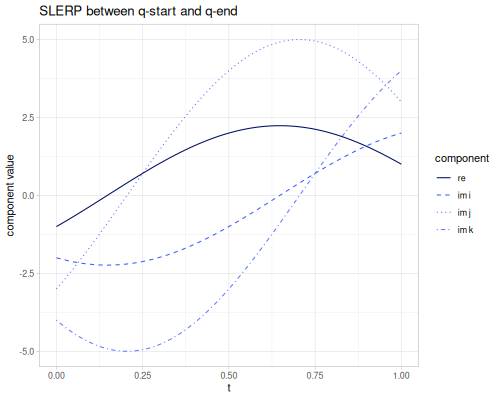

Reference

fastmath.complex

Complex numbers operations.

Complex numbers are represented using the Vec2 type defined in the fastmath.vector namespace. A complex number $z = a + bi$ corresponds to the vector (Vec2. a b).

To create a complex number, use complex, vec2, or convert from sequences/arrays using functions like fastmath.vector/seq->vec2.

The implementation correctly handles floating-point special values such as ##Inf, ##NaN, and distinguishes between +0.0 and -0.0 where necessary.

This namespace provides standard complex number operations like arithmetic (+, -, *, /), exponentiation (pow, exp, log), trigonometric functions (sin, cos, tan, etc.), and their inverses, as well as utility functions like abs, arg, conjugate, etc.

-I

z=0-i

Complex numbers

Constants

Basic operations

Predicates

Power and logarithms

Trigonometric and Hyperbolic

Quaternions

Constants

Basic operations

Predicates

Power and Logarithms

Trigonometric and Hyperbolic

Rotation Functions

Slerp

Reference

fastmath.complex

-I

I

I-

ONE

PI

TWO

ZERO

abs

acos

acosh

acot

acoth

acsc

acsch

add

adds

arg

asec

asech

asin

asinh

atan

atanh

complex

conjugate

cos

cosh

cot

coth

csc

csch

csgn

delta-eq

div

ensure-complex

exp

flip

im

imaginary?

inf?

invalid?

log

logb

muladd

mult

mult-I

mult-I-

nan?

neg

norm

normalize

pow

re

real?

reciprocal

scale

sec

sech

sin

sinh

sq

sqrt

sqrt1z

sub