Core

Collection of type hinted math macros and functions. Partially backed by Java static functions and exposed as macros. They are prepared to accept primitive long or double arguments and return long or double only.

There is a possibility to replace clojure.core functions with a selection of fastmath.core macros. Call:

• (m/use-primitive-operators) to replace functions with macros
• (m/unuse-primitive-operators) to revert replacement.

Be aware that there are some differences and fastmath.core versions shoudn’t be treated as a drop-in replacement for clojure.core versions. Also, since Clojure 1.12, always call unuse-primitive-operators at the end of the namespace.

Here is the complete list of replaced functions:

• * + - /
• > < >= <= ==
• rem quot mod
• bit-or bit-and bit-xor bit-not bit-and-not
• bit-shift-left bit-shift-right unsigned-bit-shift-right
• bit-set bit-clear bit-flip bit-test
• inc dec
• zero? neg? pos? even? odd?
• min max
• abs

(require '[fastmath.core :as m])

Basic operations

Basic math operations.

When used in an expression oprations are inlined and can accept mixture of long and double values. If all values are of long primitive type, long is returned, double otherwise.

When used in higher order function, double is returned always. To operate on long primitive type, reach for long- versions.

Defined functions

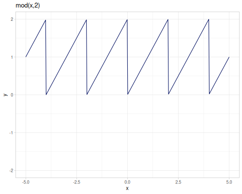
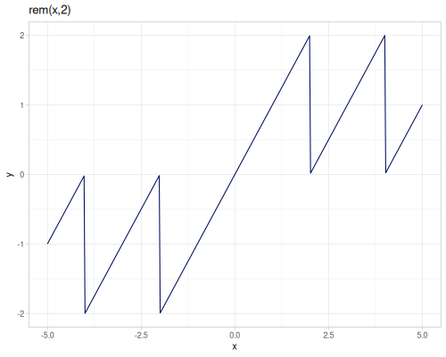
• +, -, *, /, quot
• inc, dec
• min, max, smooth-max, constrain
• rem, mod, remainder, wrap
• abs

long versions

• long-add, long-sub, long-mult, long-div, long-quot
• long-inc, long-dec
• long-min, long-max
• long-rem, long-mod
• long-abs

Arithmetics

• addition, incrementation
• subtraction, decrementation
• multiplication
• division
• absolute value

Division differences

Please note that there some differences between division in fastmath and clojure.core

• when called with one argument (double or long) m// always returns reciprocal (clojure.core// returns a ratio)
• when called on long arguments, m// is a long division (clojure.core// returns a ratio)
• m// for two long arguments is equivalent to m/quot

Examples

Addition

(m/+) ;; => 0.0
(m/+ 1 2 3 4) ;; => 10
(m/+ 1.0 2.5 3 4) ;; => 10.5
(reduce m/+ [1 2 3]) ;; => 6.0

(m/long-add) ;; => 0
(m/long-add 1 2 3 4) ;; => 10
(m/long-add 1.0 2.5 3 4) ;; => 10
(reduce m/long-add [1 2 3.5]) ;; => 6

Subtraction

[(m/- 1) (m/- 1.0)] ;; => [-1 -1.0]
(m/- 1 2 3 4) ;; => -8
(m/- 1.0 2.5 3 4) ;; => -8.5
(reduce m/- [1 2 3]) ;; => -4.0

(m/long-sub 1) ;; => -1
(m/long-sub 1 2 3 4) ;; => -8
(m/long-sub 1.0 2.5 3 4) ;; => -8
(reduce m/long-sub [1 2 3.5]) ;; => -4

Multiplication

(m/*) ;; => 1.0
(m/* 1 2 3 4) ;; => 24
(m/* 1.0 2.5 3 4) ;; => 30.0
(reduce m/* [1 2 3]) ;; => 6.0

(m/long-mult) ;; => 1
(m/long-mult 1 2 3 4) ;; => 24
(m/long-mult 1.0 2.5 3 4) ;; => 24
(reduce m/long-mult [1 2 3.5]) ;; => 6

Division

[(m// 2) (m// 2) (/ 2)] ;; => [0.5 0.5 1/2]
(m// 1 2 3 4) ;; => 0
(m// 1.0 2.5 3 4) ;; => 0.03333333333333333
(reduce m// [1 2 3]) ;; => 0.16666666666666666
(m/quot 10.5 -3) ;; => -3.0

(m/long-div 2) ;; => 0.5
(m/long-div 100 5 3) ;; => 6
(m/long-div 100.5 2.5 3) ;; => 16
(reduce m/long-div [100 2 3.5]) ;; => 16
(m/long-quot 10 -3) ;; => -3

Increment and decrement

(m/inc 4) ;; => 5
(m/inc 4.5) ;; => 5.5
(m/dec 4) ;; => 3
(m/dec 4.5) ;; => 3.5
(map m/inc [1 2 3.5 4.5]) ;; => (2.0 3.0 4.5 5.5)

(m/long-inc 4) ;; => 5
(m/long-inc 4.5) ;; => 5
(m/long-dec 4) ;; => 3
(m/long-dec 4.5) ;; => 3
(map m/long-inc [1 2 3.5 4.5]) ;; => (2 3 4 5)

Absolute value

(m/abs -3) ;; => 3
(m/long-abs -3) ;; => 3
(m/abs -3.5) ;; => 3.5
(m/long-abs -3.5) ;; => 3

Remainders

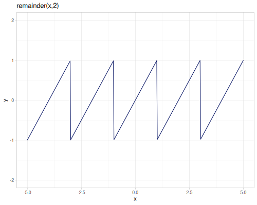
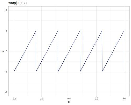
• rem and mod are the same as in clojure.core,
• remainder returns \(dividend - divisor * n\), where \(n\) is the mathematical integer closest to \(\frac{dividend}{divisor}\). Returned value is inside the \([\frac{-|divisor|}{2},\frac{|divisor|}{2}]\) range.
• wrap wraps the value to be within given interval (right open) \([a,b)\) `

Examples

(m/mod 10 4) ;; => 2
(m/mod -10.25 4.0) ;; => 1.75
(m/mod 10.25 -4.0) ;; => -1.75
(m/mod -10.25 -4.0) ;; => -2.25
(m/rem 10 4) ;; => 2
(m/rem -10.25 4.0) ;; => -2.25
(m/rem 10.25 -4.0) ;; => 2.25
(m/rem -10.25 -4.0) ;; => -2.25
(m/remainder 10 4) ;; => 2.0
(m/remainder -10.25 4.0) ;; => 1.75
(m/remainder 10.25 -4.0) ;; => -1.75
(m/remainder -10.25 -4.0) ;; => 1.75
(m/wrap -1.25 1.25 1.0) ;; => 1.0
(m/wrap -1.25 1.25 1.35) ;; => -1.15
(m/wrap -1.25 1.25 -1.25) ;; => -1.25
(m/wrap -1.25 1.25 1.25) ;; => -1.25
(m/wrap [-1.25 1.25] -1.35) ;; => 1.15

Min, max, constrain

Constrain is a macro which is equivalent to (max (min value mx) mn)

Examples

(m/min 1 2 -3) ;; => -3
(m/min 1.0 2 -3) ;; => -3.0
(m/max 1 2 -3) ;; => 2
(m/max 1.0 2 -3) ;; => 2.0
(m/constrain 10 -1 1) ;; => 1
(m/constrain -10 -1 1) ;; => -1
(m/constrain 0 -1 1) ;; => 0

Smooth maximum

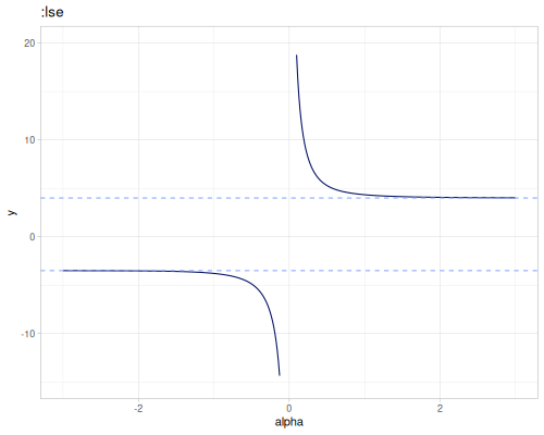
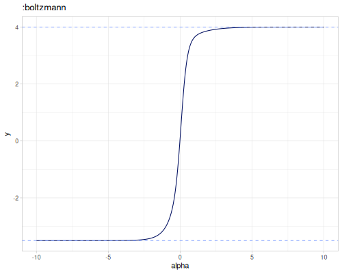
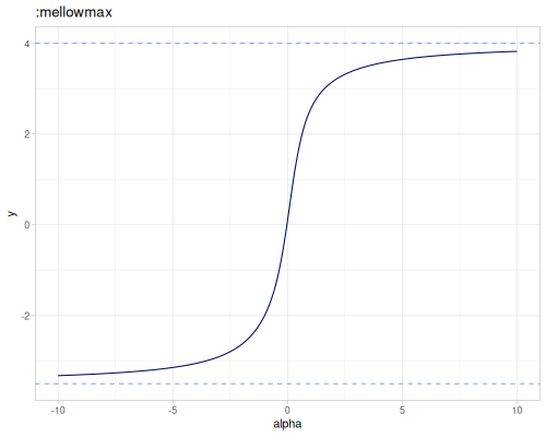
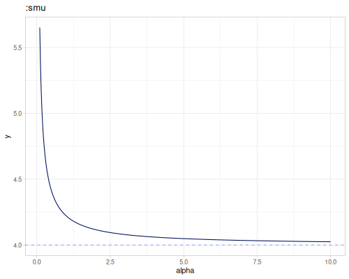
Smooth maximum is a family of functions \(\max_\alpha(xs)\) for which \(\lim_{\alpha\to\infty}\max_\alpha(xs)=\max(xs)\).

Five types of smooth maximum are defined (see wikipedia for formulas):

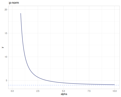
• :lse - LogSumExp (default)
• :boltzmann - Boltzmann operator, works for small alpha values
• :mellowmax
• :p-norm
• :smu - smooth maximum unit, \(\epsilon=\frac{1}{\alpha}\)

:lse, :boltzmann and :mellowmax are also smooth minimum for negative \(\alpha\) values.

The following plots show value of the smooth max for different \(\alpha\) and set of the numbers equal to [-3.5 -2 -1 0.1 3 4]. Blue dashed horizontal lines are minimum (-3.5) and maximum values (4.0).

The following plots are defined only for positive \(\alpha\).

Examples

(m/smooth-max [-3.5 -2 -1 0.1 3 4] 4.0 :lse) ;; => 4.004537523710555
(m/smooth-max [-3.5 -2 -1 0.1 3 4] -4.0 :lse) ;; => -3.500630381944282
(m/smooth-max [-3.5 -2 -1 0.1 3 4] 4.0 :boltzmann) ;; => 3.9820131397304284
(m/smooth-max [-3.5 -2 -1 0.1 3 4] -4.0 :boltzmann) ;; => -3.496176019710726
(m/smooth-max [-3.5 -2 -1 0.1 3 4] 4.0 :mellowmax) ;; => 3.5565976564035413
(m/smooth-max [-3.5 -2 -1 0.1 3 4] -4.0 :mellowmax) ;; => -3.0526905146372685
(m/smooth-max [-3.5 -2 -1 0.1 3 4] 4.0 :p-norm) ;; => 4.738284340366858
(m/smooth-max [-3.5 -2 -1 0.1 3 4] 4.0 :smu) ;; => 4.060190281957045

fma

Fused multiply-add \(fma(a,b,c)=a+bc\) is the operation implemented with better accuracy in Java 9+ and as one instruction (see more here and here). When Java 8 is used fma is replaced with direct a+bc formula.

Defined functions

• fma, muladd, negmuladd
• difference-of-products, sum-of-products

\[\operatorname{fma}(a,b,c)=\operatorname{muladd}(a,b,c)=a+bc\] \[\operatorname{negmuladd}(a,b,c)=\operatorname{fma}(-a,b,c)\]

difference-of-products (dop) and sum-of-products (sop) are using Kahan’s algorithm to avoid catastrophic cancellation.

\[\operatorname{dop}(a,b,c,d)=ab-cd=\operatorname{fma}(a,b,-cd)+\operatorname{fma}(-c,d,cd)\] \[\operatorname{sop}(a,b,c,d)=ab+cd=\operatorname{fma}(a,b,cd)+\operatorname{fma}(c,d,-cd)\]

The following example shows that \(x^2-y^2\) differs from the best floating point approximation which is equal 1.8626451518330422e-9.

(let [x (m/inc (m/pow 2 -29))
      y (m/inc (m/pow 2 -30))]
  {:proper-value (m/difference-of-products x x y y)
   :wrong-value (m/- (m/* x x) (m/* y y))})

{:proper-value 1.8626451518330422E-9, :wrong-value 1.862645149230957E-9}

Examples

(m/fma 3 4 5) ;; => 17.0
(m/muladd 3 4 5) ;; => 17.0
(m/negmuladd 3 4 5) ;; => -7.0
(m/difference-of-products 3 3 4 4) ;; => -7.0
(m/sum-of-products 3 3 4 4) ;; => 25.0

Rounding

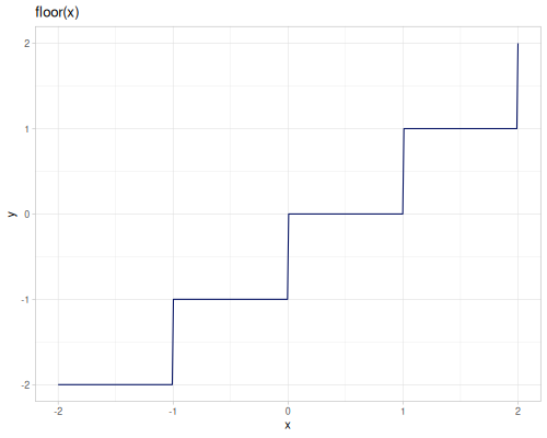
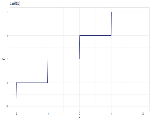
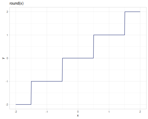
Various rounding functions.

Defined functions

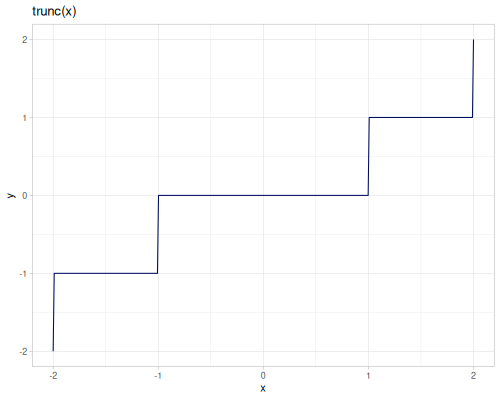
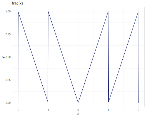
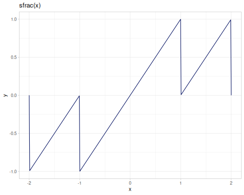
• floor, ceil
• round, round-even, rint, approx, trunc, itrunc
• qfloor, qceil, qround
• frac, sfrac
• round-up-pow2

• floor, ceil and rint accept additional argument, scale, which allows to round to the nearest multiple of scale.
• round returns long while rint returns double
• round-even performs IEEE / IEC rounding (even-odd or bankers’ rounding)
• approx rounds number to the given number of digits, uses bigdec
• trunc returns integer part of a number, frac returns fractional part
• trunc returns double while itrunc returns long
• sfrac keeps sign of the argument
• qfloor, qceil and qround are implemented using casting to long
• round-up-pow2 rounds to the lowest power of 2 greater than an argument, \(2^{\left\lceil{\log_2{x}}\right\rceil}\), returns long.

Examples

(map m/floor [-10.5 10.5]) ;; => (-11.0 10.0)
(m/floor 10.5 4.0) ;; => 8.0
(map m/ceil [-10.5 10.5]) ;; => (-10.0 11.0)
(m/ceil 10.5 4.0) ;; => 12.0
(map m/rint [-10.51 -10.5 -10.49 10.49 10.5 10.51]) ;; => (-11.0 -10.0 -10.0 10.0 10.0 11.0)
(m/rint 10.5 4.0) ;; => 12.0
(m/rint 10.591 0.1) ;; => 10.600000000000001
(map m/round [-10.51 -10.5 -10.49 10.49 10.5 10.51]) ;; => (-11 -10 -10 10 11 11)
(map m/round-even [-10.51 -10.5 -10.49 10.49 10.5 10.51]) ;; => (-11 -10 -10 10 10 11)
(map m/qfloor [-10.5 10.5]) ;; => (-11 10)
(map m/qceil [-10.5 10.5]) ;; => (-10 11)
(map m/qround [-10.51 -10.5 -10.49 10.49 10.5 10.51]) ;; => (-11 -11 -10 10 11 11)
(map m/trunc [-10.591 10.591]) ;; => (-10.0 10.0)
(map m/itrunc [-10.591 10.591]) ;; => (-10 10)
(m/approx 10.591) ;; => 10.59
(m/approx 10.591 1) ;; => 10.6
(m/approx 10.591 0) ;; => 11.0
(m/approx -10.591) ;; => -10.59
(m/approx -10.591 1) ;; => -10.6
(m/approx -10.591 0) ;; => -11.0
(map m/frac [-10.591 10.591]) ;; => (0.5909999999999993 0.5909999999999993)
(map m/sfrac [-10.591 10.591]) ;; => (-0.5909999999999993 0.5909999999999993)
(map m/round-up-pow2 (range 10)) ;; => (0 1 2 4 4 8 8 8 8 16)

The difference between rint and round. round is bounded by minimum and maximum long values.

(m/rint 1.23456789E30) ;; => 1.23456789E30
(m/round 1.23456789E30) ;; => 9223372036854775807

Sign

Sign of the number.

Defined functions

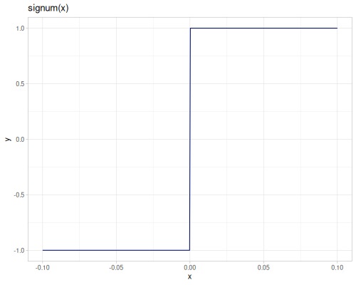
• signum and sgn
• copy-sign

\[\operatorname{signum}(x)=\begin{cases} -1 & x<0 \\ 1 & x>0 \\ 0 & x=0 \end{cases}\]

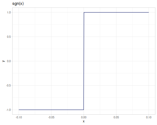
\[\operatorname{sgn}(x)=\begin{cases} -1 & x<0 \\ 1 & x\geq 0 \end{cases}\]

copy-sign sets the sign of the second argument to the first. Please note that -0.0 is negative and 0.0 is positive.

\[\operatorname{copy-sign}(x,y)=\begin{cases} |x| & y>0 \lor y=0.0\\ -|x| & y<0 \lor y=-0.0 \end{cases}\]

Examples

(m/signum -2.5) ;; => -1.0
(m/signum 2.5) ;; => 1.0
(m/sgn -2.5) ;; => -1.0
(m/sgn 2.5) ;; => 1.0
(m/signum 0) ;; => 0.0
(m/sgn 0) ;; => 1.0
(m/copy-sign 123 -10) ;; => -123.0
(m/copy-sign -123 10) ;; => 123.0
(m/copy-sign 123 -0.0) ;; => -123.0
(m/copy-sign -123 0.0) ;; => 123.0

Comparison and Predicates

Various predicates and comparison functions

Defined functions

• ==, eq, not==, <, >, <=, >=
• approx-eq, approx=, delta-eq, delta=
• zero?, negative-zero?, near-zero?, one?
• neg?, pos?, not-neg?, not-pos?
• even?, odd?
• integer?
• nan?, inf?, pos-inf?, neg-inf?, invalid-double?, valid-double?
• between?, between-?

Comparison

Comparison functions operate on primitive values and can handle multiple arguments, chaining the comparison (e.g., (m/< 1 2 3) is equivalent to (and (m/< 1 2) (m/< 2 3))).

Standard comparisons:

• ==, eq: Primitive equality. Note that (m/== 1.0 1) is true. Multi-arity checks if the first argument is equal to all subsequent arguments.
• not==: Primitive inequality. Multi-arity checks if all arguments are pairwise unique.
• <, >, <=, >=: Standard primitive inequalities. Multi-arity checks if the values are monotonically increasing/decreasing.

Approximate equality:

• approx-eq, approx=: Checks for equality after rounding to a specified number of decimal digits. Can be inaccurate.
• delta-eq, delta=: Checks if the absolute difference between two numbers is within a given tolerance (absolute and/or relative). This is the recommended way to compare floating-point numbers for near equality
  • With absolute tolerance: \(|a - b| < \text{abs-tol}\)
  • With absolute and relative tolerance: \(|a - b| < \max(\text{abs-tol}, \text{rel-tol} \cdot \max(|a|, |b|))\)

Range checks:

• between?: Checks if a value is within a closed interval \([a, b]\), i.e., \(a \le \text{value} \le b\).
• between-?: Checks if a value is within a half-open interval \((a, b]\), i.e., \(a < \text{value} \le b\).

Examples

(m/== 1.0 1) ;; => true
(m/== 1.0 2) ;; => false
(m/== 1 1 2 3 4) ;; => false
(m/eq 1.0 1) ;; => true
(m/not== 1.0 1) ;; => false
(m/not== 1.0 2) ;; => true
(m/not== 1 2 3 4) ;; => true
(m/not== 1 2 3 1 4) ;; => false
(m/< 1.0 1) ;; => false
(m/< 1.0 2) ;; => true
(m/< 2 1.0) ;; => false
(m/< 1 2 3 4 10) ;; => true
(m/< 10 4 3 2 1) ;; => false
(m/<= 1.0 1) ;; => true
(m/<= 1.0 2) ;; => true
(m/<= 2 1.0) ;; => false
(m/> 1.0 1) ;; => false
(m/> 1.0 2) ;; => false
(m/> 2 1.0) ;; => true
(m/> 1 2 3 4 10) ;; => false
(m/> 10 4 3 2 1) ;; => true
(m/>= 1.0 1) ;; => true
(m/>= 1.0 2) ;; => false
(m/>= 2 1.0) ;; => true
(m/between? -1 1 -1) ;; => true
(m/between? -1 1 0) ;; => true
(m/between? -1 1 1) ;; => true
(m/between-? -1 1 -1) ;; => false
(m/between-? -1 1 0) ;; => true
(m/between-? -1 1 1) ;; => true

Examples

(m/approx-eq 10 10.01) ;; => false
(m/approx-eq 10 10.001) ;; => true
(m/approx-eq 10 10.01 1) ;; => true
(m/approx-eq 10 10.001 5) ;; => false
(m/delta-eq 10 10.01) ;; => false
(m/delta-eq 10 10.01 0.1) ;; => true
(m/delta-eq 1.0E-6 1.01E-6) ;; => true
(m/delta-eq 1.0E-6 1.01E-6 1.0E-8) ;; => false
(m/delta-eq 1.0E-6 1.01E-6 1.0E-8 0.01) ;; => true

Predicates

Basic predicates for common number properties:

• zero?: Checks if value is 0 or 0.0.
• negative-zero?: Checks specifically for the floating point -0.0.
• near-zero?: Checks if absolute value is within absolute and/or relative tolerance of zero: \(|x| < \text{abs-tol}\) or \(|x| < \max(\text{abs-tol}, \text{rel-tol} \cdot |x|)\).
• one?: Checks if value is 1 or 1.0.
• neg?: Checks if value is \(< 0\).
• pos?: Checks if value is \(> 0\).
• not-neg?: Checks if value is \(\ge 0\).
• not-pos?: Checks if value is \(\le 0\).
• even?: Checks if a long is even.
• odd?: Checks if a long is odd.
• integer?: Checks if a number (long or double) has a zero fractional part.

Examples

(m/zero? 0) ;; => true
(m/zero? 0.0) ;; => true
(m/zero? -0.0) ;; => true
(m/zero? 1) ;; => false
(m/negative-zero? 0.0) ;; => false
(m/negative-zero? -0.0) ;; => true
(m/one? 1) ;; => true
(m/one? 1.0) ;; => true
(m/neg? -1) ;; => true
(m/neg? 0) ;; => false
(m/neg? 1.0) ;; => false
(m/pos? -1) ;; => false
(m/pos? 0) ;; => false
(m/pos? 1.0) ;; => true
(m/not-neg? -1) ;; => false
(m/not-neg? 0) ;; => true
(m/not-neg? 1.0) ;; => true
(m/not-pos? -1) ;; => true
(m/not-pos? 0) ;; => true
(m/not-pos? 1.0) ;; => false
(m/even? 0) ;; => true
(m/even? 1) ;; => false
(m/even? 2) ;; => true
(m/odd? 0) ;; => false
(m/odd? 1) ;; => true
(m/odd? 2) ;; => false
(m/integer? 1) ;; => true
(m/integer? 1.0) ;; => true
(m/integer? 1.1) ;; => false

Predicates for floating point special values:

• nan?: Checks if value is Not-a-Number (NaN).
• inf?: Checks if value is positive or negative infinity (Inf or -Inf).
• pos-inf?: Checks if value is positive infinity (Inf).
• neg-inf?: Checks if value is negative infinity (-Inf).
• invalid-double?: Checks if value is not a finite double (NaN or ±Inf).
• valid-double?: Checks if value is a finite double (not NaN or ±Inf).

Examples

(m/nan? ##NaN) ;; => true
(m/nan? ##Inf) ;; => false
(m/nan? ##-Inf) ;; => false
(m/nan? 1) ;; => false
(m/inf? ##NaN) ;; => false
(m/inf? ##Inf) ;; => true
(m/inf? ##-Inf) ;; => true
(m/inf? 1) ;; => false
(m/pos-inf? ##NaN) ;; => false
(m/pos-inf? ##Inf) ;; => true
(m/pos-inf? ##-Inf) ;; => false
(m/pos-inf? 1) ;; => false
(m/neg-inf? ##NaN) ;; => false
(m/neg-inf? ##Inf) ;; => false
(m/neg-inf? ##-Inf) ;; => true
(m/neg-inf? 1) ;; => false
(m/valid-double? ##NaN) ;; => false
(m/valid-double? ##Inf) ;; => false
(m/valid-double? ##-Inf) ;; => false
(m/valid-double? 1) ;; => true
(m/invalid-double? ##NaN) ;; => true
(m/invalid-double? ##Inf) ;; => true
(m/invalid-double? ##-Inf) ;; => true
(m/invalid-double? 1) ;; => false

Trigonometry

Trigonometric (with historical variants) and hyperbolic functions.

Defined functions

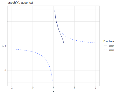
• radians, degrees
• sin, cos, tan, cot, sec, csc
• qsin, qcos
• sinpi, cospi, tanpi, cotpi, secpi, cscpi
• asin, acos, atan, atan2, acot, asec, acsc
• sinh, cosh, tanh, coth, sech, scsh
• asinh, acosh, atanh, acoth, asech, ascsh
• crd, acrd
• versin, coversin, vercos, covercos
• aversin, acoversin, avercos, acovercos
• haversin, hacoversin, havercos, hacovercos
• ahaversin, ahacoversin, ahavercos, ahacovercos
• exsec, excsc
• aexsec, aexcsc
• sinc

Angle conversion

Convert between radians and degrees

• radians(deg): Converts an angle from degrees to radians. \[\text{radians} = \text{degrees} \cdot \frac{\pi}{180^\circ}\]
• degrees(rad): Converts an angle from radians to degrees. \[\text{degrees} = \text{radians} \cdot \frac{180^\circ}{\pi}\]

Examples

(m/radians 180) ;; => 3.141592653589793
(m/degrees m/PI) ;; => 180.0
(m/radians 90) ;; => 1.5707963267948966
(m/degrees m/HALF_PI) ;; => 90.0

Trigonometric

Standard trigonometric functions:

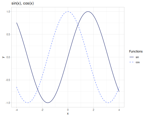
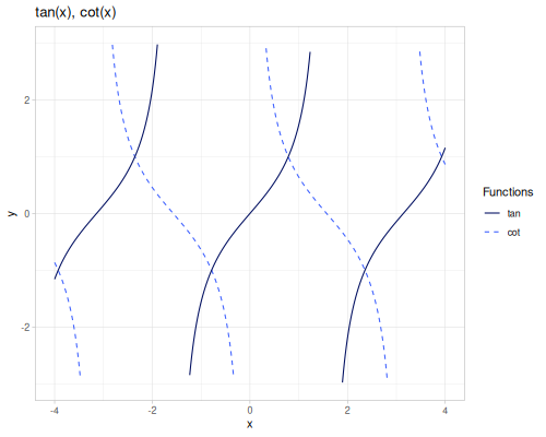
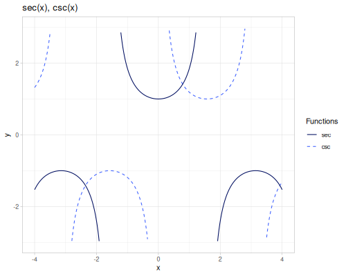
• sin(x): Sine of x.
• cos(x): Cosine of x.
• tan(x): Tangent of x, \(\tan(x) = \frac{\sin(x)}{\cos(x)}\).
• cot(x): Cotangent of x, \(\cot(x) = \frac{1}{\tan(x)}\).
• sec(x): Secant of x, \(\sec(x) = \frac{1}{\cos(x)}\).
• csc(x): Cosecant of x, \(\csc(x) = \frac{1}{\sin(x)}\).

Examples

(m/sin m/HALF_PI) ;; => 1.0
(m/cos m/PI) ;; => -1.0
(m/tan m/QUARTER_PI) ;; => 0.9999999999999997
(m/cot m/HALF_PI) ;; => 6.12323399538461E-17
(m/sec 0.0) ;; => 1.0
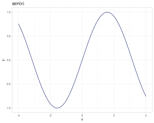
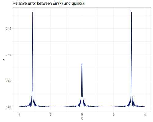
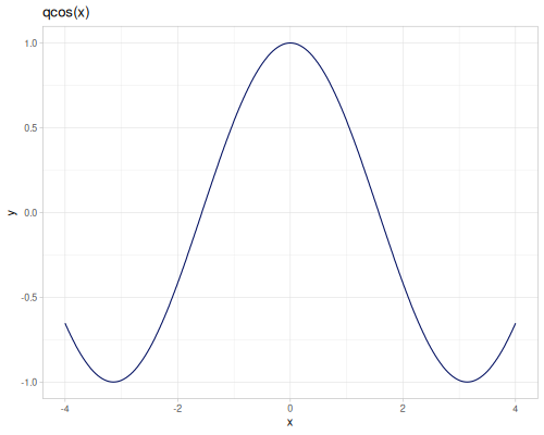
(m/csc m/HALF_PI) ;; => 1.0

Quick trigonometric functions:

• qsin(x): Fast, less accurate sine.
• qcos(x): Fast, less accurate cosine.

Examples

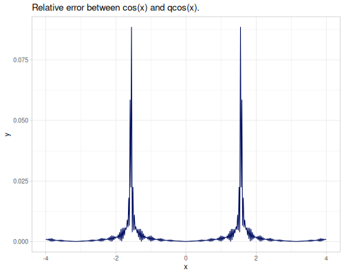(m/qsin 0.1) ;; => 0.10106986275482788
(m/sin 0.1) ;; => 0.09983341664682818
(m/qcos 0.1) ;; => 0.9948793307948056
(m/cos 0.1) ;; => 0.9950041652780257

Pi-scaled trigonometric functions:

• sinpi(x): Sine of \(\pi x\), \(\sin(\pi x)\).
• cospi(x): Cosine of \(\pi x\), \(\cos(\pi x)\).
• tanpi(x): Tangent of \(\pi x\), \(\tan(\pi x)\).
• cotpi(x): Cotangent of \(\pi x\), \(\cot(\pi x)\).
• secpi(x): Secant of \(\pi x\), \(\sec(\pi x)\).
• cscpi(x): Cosecant of \(\pi x\), \(\csc(\pi x)\).

Examples

(m/sinpi 0.5) ;; => 1.0
(m/cospi 1) ;; => -1.0
(m/tanpi 0.25) ;; => 0.9999999999999997
(m/cotpi 0.5) ;; => 6.12323399538461E-17
(m/secpi 0) ;; => 1.0
(m/cscpi 0.5) ;; => 1.0

Inverse trigonometric

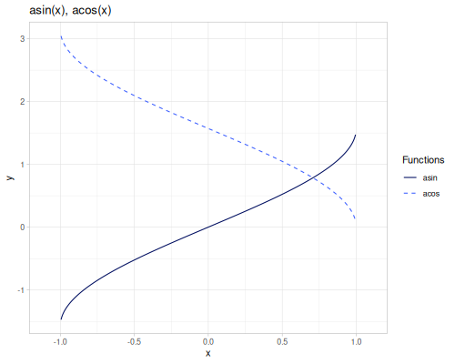
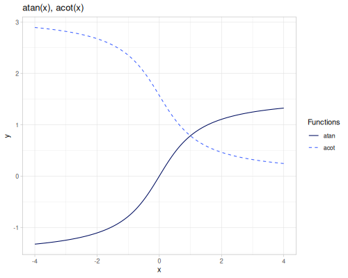
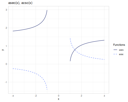
Inverse trigonometric functions:

• asin(x): Arcsine of x, \(\arcsin(x)\).
• acos(x): Arccosine of x, \(\arccos(x)\).
• atan(x): Arctangent of x, \(\arctan(x)\).
• atan2(y, x): Arctangent of \(\frac{y}{x}\), returning the angle in the correct quadrant.
• acot(x): Arccotangent of x, \(\operatorname{arccot}(x) = \frac{\pi}{2} - \arctan(x)\).
• asec(x): Arcsecant of x, \(\operatorname{arcsec}(x) = \arccos(\frac{1}{x})\).
• acsc(x): Arccosecant of x, \(\operatorname{arccsc}(x) = \arcsin(\frac{1}{x})\).

Examples

(m/asin 1) ;; => 1.5707963267948966
(m/acos -1) ;; => 3.141592653589793
(m/atan 1) ;; => 0.7853981633974483
(m/acot 0) ;; => 1.5707963267948966
(m/asec 1) ;; => 0.0
(m/acsc 1) ;; => 1.5707963267948966
(m/atan2 1 1) ;; => 0.7853981633974483

Special

sinc(x): Sinc function: \(\operatorname{sinc}(x) = \frac{\sin(\pi x)}{\pi x}\) for \(x \ne 0\), and \(1\) for \(x=0\).

Examples

(m/sinc 0.0) ;; => 1.0
(m/sinc 1.0) ;; => 3.898171832295186E-17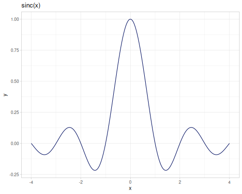

Hyperbolic

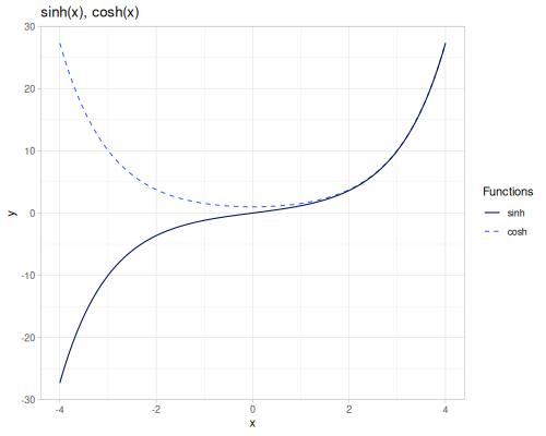
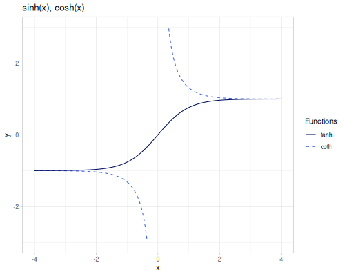
Hyperbolic functions

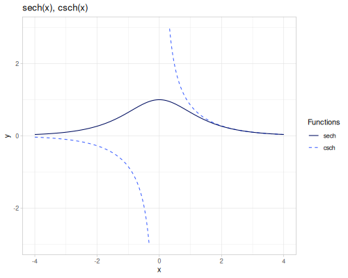
• sinh(x): Hyperbolic sine, \(\sinh(x) = \frac{e^x - e^{-x}}{2}\).
• cosh(x): Hyperbolic cosine, \(\cosh(x) = \frac{e^x + e^{-x}}{2}\).
• tanh(x): Hyperbolic tangent, \(\tanh(x) = \frac{\sinh(x)}{\cosh(x)}\).
• coth(x): Hyperbolic cotangent, \(\coth(x) = \frac{1}{\tanh(x)}\).
• sech(x): Hyperbolic secant, \(\operatorname{sech}(x) = \frac{1}{\cosh(x)}\).
• csch(x): Hyperbolic cosecant, \(\operatorname{csch}(x) = \frac{1}{\sinh(x)}\).

(m/sinh 0) ;; => 0.0
(m/cosh 0) ;; => 1.0
(m/tanh 0) ;; => 0.0
(m/coth 1) ;; => 1.3130352854993315
(m/sech 0) ;; => 1.0
(m/csch 1) ;; => 0.8509181282393214

Inverse hyperbolic

Inverse hyperbolic functions:

• asinh(x): Area hyperbolic sine, \(\operatorname{arsinh}(x) = \ln(x + \sqrt{x^2 + 1})\).
• acosh(x): Area hyperbolic cosine, \(\operatorname{arcosh}(x) = \ln(x + \sqrt{x^2 - 1})\) for \(x \ge 1\).
• atanh(x): Area hyperbolic tangent, \(\operatorname{artanh}(x) = \frac{1}{2} \ln(\frac{1 + x}{1 - x})\) for \(-1 < x < 1\).
• acoth(x): Area hyperbolic cotangent, \(\operatorname{arcoth}(x) = \operatorname{artanh}(\frac{1}{x})\).
• asech(x): Area hyperbolic secant, \(\operatorname{arsech}(x) = \operatorname{arcosh}(\frac{1}{x})\).
• acsch(x): Area hyperbolic cosecant, \(\operatorname{arcsch}(x) = \operatorname{arsinh}(\frac{1}{x})\).

Examples

(m/asinh 0) ;; => 0.0
(m/acosh 1) ;; => 0.0
(m/atanh 0) ;; => 0.0
(m/acoth 2) ;; => 0.5493061443340548
(m/asech 1) ;; => 0.0
(m/acsch 1) ;; => 0.8813735870195429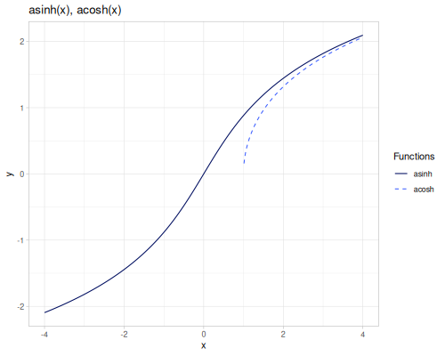

Historical

Historical/Specific trigonometric functions:

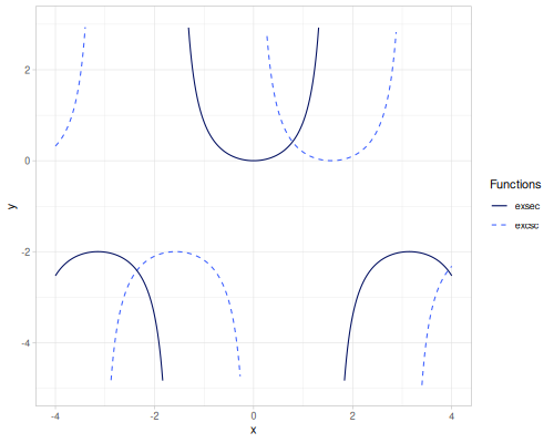
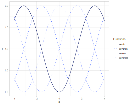
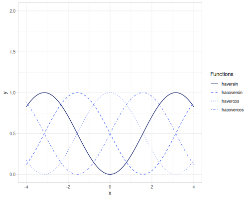
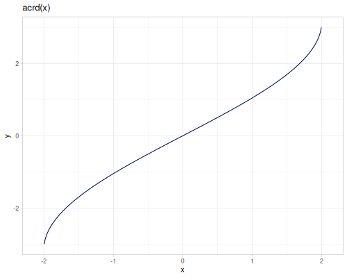
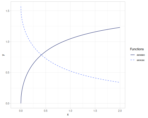
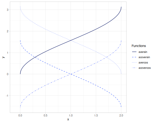
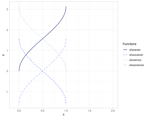
• crd(x): Chord, \(\operatorname{crd}(x) = 2 \sin(\frac{x}{2})\).
• acrd(x): Inverse chord, \(\operatorname{acrd}(x) = 2 \arcsin(\frac{x}{2})\).
• versin(x): Versine, \(\operatorname{versin}(x) = 1 - \cos(x)\).
• coversin(x): Coversine, \(\operatorname{coversin}(x) = 1 - \sin(x)\).
• vercos(x): Vercosine, \(\operatorname{vercos}(x) = 1 + \cos(x)\).
• covercos(x): Covercosine, \(\operatorname{covercos}(x) = 1 + \sin(x)\).
• haversin(x) / haversine(x): Haversine, \(\operatorname{hav}(x) = \sin^2(\frac{x}{2}) = \frac{1 - \cos(x)}{2}\). Also computes the haversine value for pairs of geographic coordinates.
• hacoversin(x): Hacoversine, \(\operatorname{hacov}(x) = \frac{1 - \sin(x)}{2}\).
• havercos(x): Havercosine, \(\operatorname{haver}(x) = \frac{1 + \cos(x)}{2}\).
• hacovercos(x): Hacovercosine, \(\operatorname{hacover}(x) = \frac{1 + \sin(x)}{2}\).
• exsec(x): Exsecant, \(\operatorname{exsec}(x) = \sec(x) - 1\).
• excsc(x): Excosecant, \(\operatorname{excsc}(x) = \csc(x) - 1\).
• aversin(x): Arc versine, \(\operatorname{aversin}(x) = \arccos(1 - x)\).
• acoversin(x): Arc coversine, \(\operatorname{acoversin}(x) = \arcsin(1 - x)\).
• avercos(x): Arc vercosine, \(\operatorname{avercos}(x) = \arccos(x - 1)\).
• acovercos(x): Arc covercosine, \(\operatorname{acovercos}(x) = \arcsin(x - 1)\).
• ahaversin(x): Arc haversine, \(\operatorname{ahav}(x) = \arccos(1 - 2x)\).
• ahacoversin(x): Arc hacoversine, \(\operatorname{ahacov}(x) = \arcsin(1 - 2x)\).
• ahavercos(x): Arc havercosine, \(\operatorname{ahaver}(x) = \arccos(2x - 1)\).
• ahacovercos(x): Arc hacovercosine, \(\operatorname{ahacover}(x) = \arcsin(2x - 1)\).
• aexsec(x): Arc exsecant, \(\operatorname{aexsec}(x) = \operatorname{arcsec}(1 + x)\).
• aexcsc(x): Arc excosecant, \(\operatorname{aexcsc}(x) = \operatorname{arccsc}(1 + x)\).

Examples

(m/crd m/HALF_PI) ;; => 1.414213562373095
(m/versin m/HALF_PI) ;; => 0.9999999999999999
(m/coversin m/PI) ;; => 0.9999999999999999
(m/vercos m/HALF_PI) ;; => 1.0
(m/covercos m/PI) ;; => 1.0000000000000002
(m/haversin m/HALF_PI) ;; => 0.49999999999999994
(m/hacoversin m/PI) ;; => 0.49999999999999994
(m/havercos m/HALF_PI) ;; => 0.5
(m/hacovercos m/PI) ;; => 0.5000000000000001
(m/exsec m/PI) ;; => -2.0
(m/excsc m/HALF_PI) ;; => 0.0
(m/acrd 2.0) ;; => 3.141592653589793
(m/aversin 1.0) ;; => 1.5707963267948966
(m/acoversin 0.0) ;; => 1.5707963267948966
(m/avercos 1.0) ;; => 1.5707963267948966
(m/acovercos 0.0) ;; => -1.5707963267948966
(m/ahaversin 1.0) ;; => 3.141592653589793
(m/ahacoversin 0.0) ;; => 1.5707963267948966
(m/ahavercos 0.0) ;; => 3.141592653589793
(m/ahacovercos 1.0) ;; => 1.5707963267948966
(m/aexsec -2.0) ;; => 3.141592653589793
(m/aexcsc 0.0) ;; => 1.5707963267948966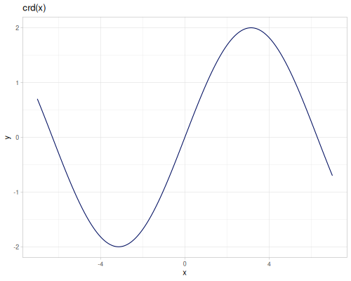

The haversine formula for calculating the square of half the chord length between two points \((\phi_1, \lambda_1)\) and \((\phi_2, \lambda_2)\) on a sphere (where \(\phi\) is latitude and \(\lambda\) is longitude, in radians) is:

\[ a = \sin^2\left(\frac{\phi_2 - \phi_1}{2}\right) + \cos(\phi_1) \cos(\phi_2) \sin^2\left(\frac{\lambda_2 - \lambda_1}{2}\right) \]

In this formula: * \(a\) is the square of half the chord length of the great-circle arc. * \(\phi_1, \phi_2\) are the latitudes of the two points. * \(\lambda_1, \lambda_2\) are the longitudes of the two points.

The actual great-circle distance \(d\) between the points on a sphere of radius \(R\) is then given by: \[ d = R \cdot 2 \arcsin(\sqrt{a}) \]

The fastmath.core/haversin function with four arguments [lat1 lon1 lat2 lon2] calculates the value \(a\). The fastmath.core/haversine-dist function then calculates the distance \(d\) assuming \(R=1\).

Let’s calculate haversin value for two lat/lon points in degrees [38.898N, 77.037E] (White House) and [48.858N, 2.294W] (Eiffel Tower).

(m/haversin (m/radians 38.898) (m/radians 77.037) (m/radians 48.858) (m/radians -2.294))

0.2161581789280517

Which is equivalent to a distance in km on Earth:

(* 6371.2
   (m/haversine-dist (m/radians 38.898) (m/radians 77.037) (m/radians 48.858) (m/radians -2.294)))

6161.63145620435

Power and logarithms

This section covers exponential, logarithmic, and power functions, including various specialized and numerically stable variants.

Defined functions

• exp, exp2, exp10, qexp
• ln, log, logb, log2, log10, qlog
• expm1, exprel, xexpx, xexpy, cexpexp, expexp
• log1p, log1pexp, log1mexp, log2mexp, log1psq, logexpm1,log1pmx, logmxp1
• xlogx, xlogy, xlog1py, cloglog, loglog, logcosh
• logaddexp, logsubexp, logsumexp, log2int
• sigmoid, logit
• sqrt, cbrt, sq, cb
• safe-sqrt, qsqrt, rqsqrt
• pow, spow, fpow, qpow, mpow, tpow, pow2, pow3, pow10
• low-2-exp, high-2-exp, low-exp, high-exp

Exponents

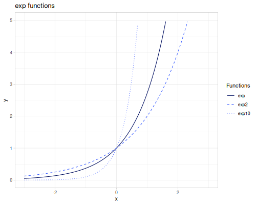
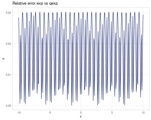
• exp(x): Natural exponential function \(e^x\).
• exp2(x): Base-2 exponential function \(2^x\).
• exp10(x): Base-10 exponential function \(10^x\).
• qexp(x): Fast, less accurate version of `exp(x)$.

Examples

(m/exp 1) ;; => 2.7182818284590455
(m/exp2 3) ;; => 8.0
(m/exp10 2) ;; => 100.0
(m/qexp 1.0) ;; => 2.799318313598633

Logarithms

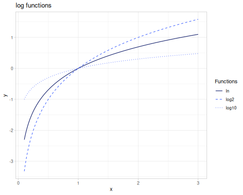
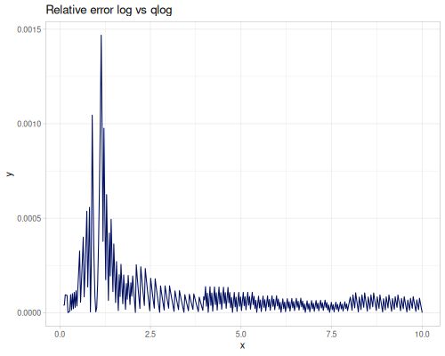
• ln(x): Natural logarithm \(\ln(x)\). Alias for log(x) with one argument.
• log(x): Natural logarithm \(\ln(x)\). With two arguments, computes \(\log_b(x)\).
• logb(b, x): Logarithm of \(x\) with base \(b\), \(\log_b(x)\).
• log2(x): Base-2 logarithm \(\log_2(x)\).
• log2int(x): Integer base-2 logarithm, related to the exponent of the floating point representation. Returns long.
• log10(x): Base-10 logarithm \(\log_{10}(x)\).
• qlog(x): Fast, less accurate version of `log(x)$.

Examples

(m/ln 10) ;; => 2.302585092994046
(m/log 10) ;; => 2.302585092994046
(m/log 2 8) ;; => 3.0
(m/logb 2 8) ;; => 3.0
(m/log2 8) ;; => 2.9999999999999996
(m/log2int 8) ;; => 3
(m/log2int 7.1) ;; => 3
(m/log10 100) ;; => 2.0
(m/qlog 10.0) ;; => 2.3025850929940455

Specialized Log/Exp functions

These functions provide numerically stable computations for expressions involving exp and log especially for small or large arguments.

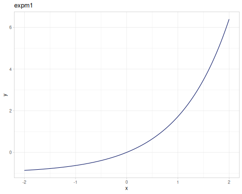
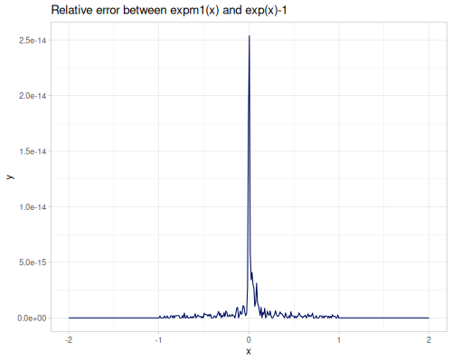
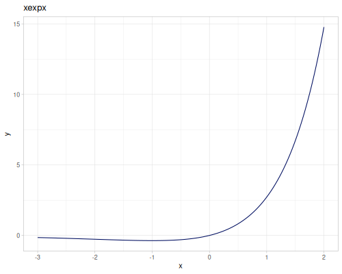
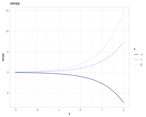
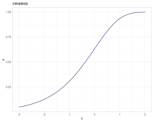
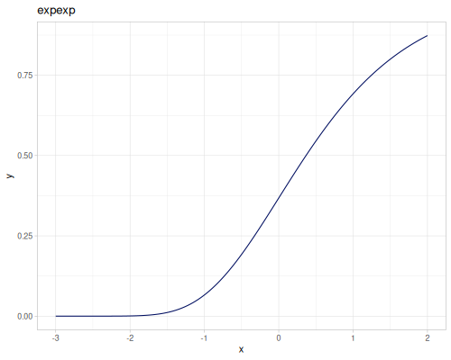
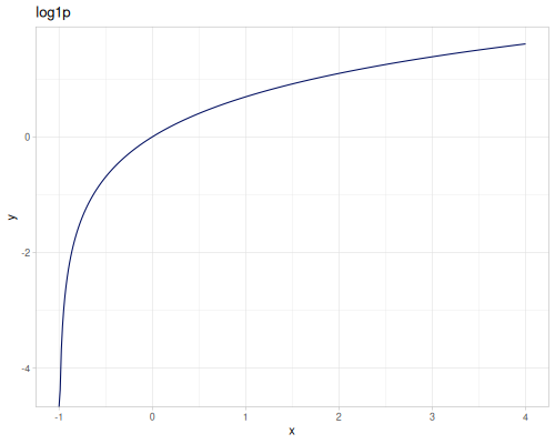
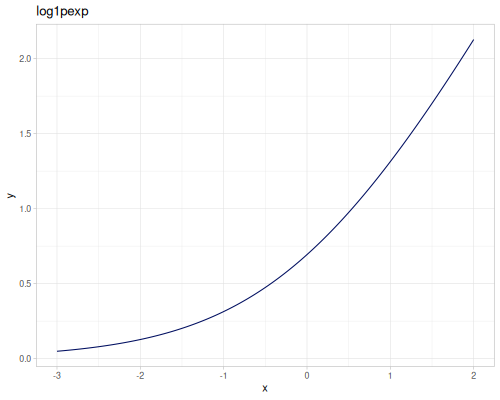
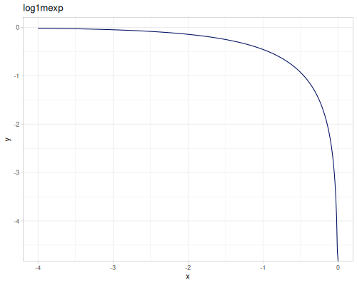
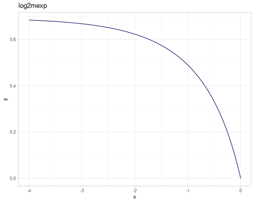
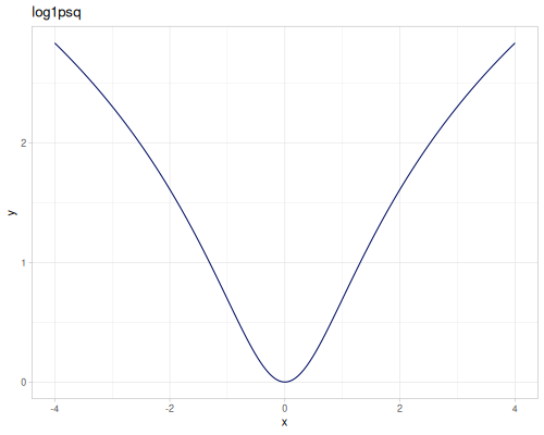
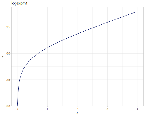
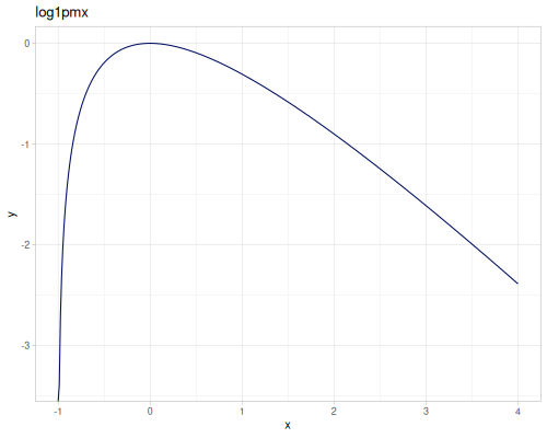
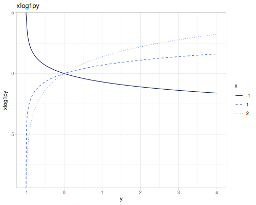
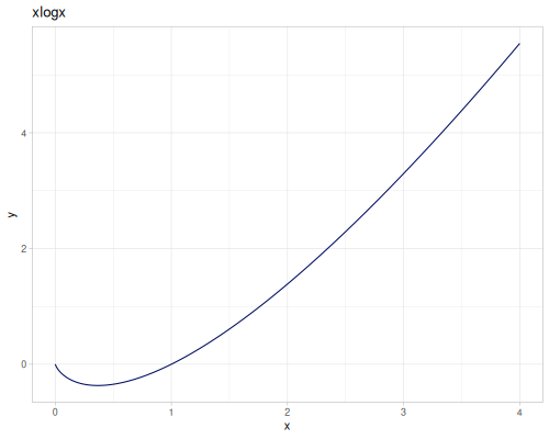
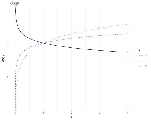
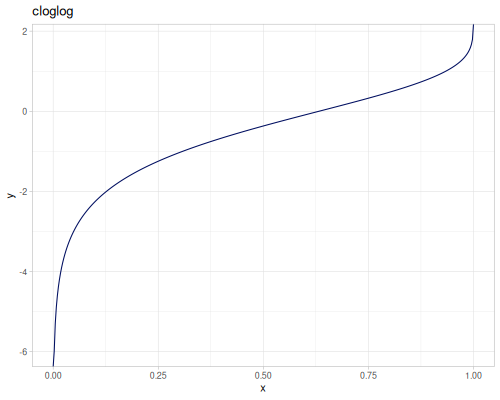
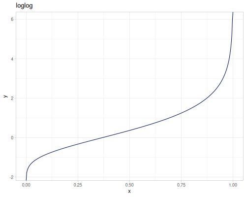
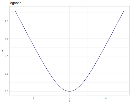
• expm1(x): \(e^x - 1\), computed accurately for small \(x\).
• exprel(x): \((e^x - 1)/x\), computed accurately for small \(x\). Returns 1 for \(x=0\).
• xexpx(x): \(x e^x\).
• xexpy(x,y): \(x e^y\).
• cexpexp(x): \(1-e^{-e^x}\), inverse of cloglog.
• expexp(x): \(e^{-e^{-x}}\), inverse of loglog.
• log1p(x): \(\ln(1+x)\), computed accurately for small \(x\).
• log1pexp(x): \(\ln(1+e^x)\).
• log1mexp(x): \(\ln(1-e^x)\), for \(x < 0\).
• log2mexp(x): \(\ln(2-e^x)\).
• log1psq(x): \(\ln(1+x^2)\), computed accurately for small \(x\).
• logexpm1(x): \(\ln(e^x - 1)\).
• log1pmx(x): \(\ln(1+x)-x\), computed accurately for small \(x\).
• logmxp1(x): \(\ln(x)-x+1\), computed accurately for \(x\) near 1.
• xlogx(x): \(x \ln(x)\). Returns 0 for \(x=0\).
• xlogy(x, y): \(x \ln(y)\). Returns 0 for \(x=0\).
• xlog1py(x, y): \(x \ln(1+y)\). Returns 0 for \(x=0\).
• cloglog(x): \(\ln(-\ln(1-x))\). Used in complementary log-log models.
• loglog(x): \(-\ln(-\ln(x))\).
• logcosh(x): \(\ln(\cosh(x))\).

Examples

(m/expm1 1.0E-9) ;; => 1.0000000005000001E-9
(m/exprel 1.0E-9) ;; => 1.0000000005000001E-9
(m/xexpx 0.5) ;; => 0.8243606353500641
(m/xexpy 0.5 -0.5) ;; => 0.3032653298563167
(m/cexpexp 1.0) ;; => 0.9340119641546875
(m/expexp 1.0) ;; => 0.6922006275553464
(m/log1p 1.0E-9) ;; => 9.999999995E-10
(m/log1pexp 0) ;; => 0.6931471805599453
(m/log1mexp -1) ;; => -0.458675145387082
(m/log2mexp -1) ;; => 0.4898801256447501
(m/log1psq 1.0E-5) ;; => 9.999999999500002E-11
(m/logexpm1 1) ;; => 0.5413248546129182
(m/log1pmx 1) ;; => -0.3068528194400547
(m/xlogx 2) ;; => 1.3862943611198906
(m/xlogy 2 5) ;; => 3.2188758248682006
(m/xlog1py 0.5 -0.5) ;; => -0.34657359027997264
(m/cloglog 0.5) ;; => -0.36651292058166435
(m/loglog 0.5) ;; => 0.36651292058166435
(m/logcosh 1) ;; => 0.4337808304830272

Log-sum-exp

These functions are used for numerically stable computation of sums and differences of exponents.

• logaddexp(x, y): \(\ln(e^x + e^y)\).
• logsubexp(x, y): \(\ln(|e^x - e^y|)\).
• logsumexp(xs): \(\ln(\sum_{i} e^{x_i})\).

Examples

(m/logaddexp 0 0) ;; => 0.6931471805599453
(m/logaddexp 100 100) ;; => 100.69314718055995
(m/logsubexp 0 0) ;; => ##-Inf
(m/logsubexp 100 99) ;; => 99.54132485461292
(m/logsumexp [0 0 0]) ;; => 1.0986122886681098
(m/logsumexp [100 100 100]) ;; => 101.09861228866811

Sigmoid and Logit

Functions used in statistics and machine learning.

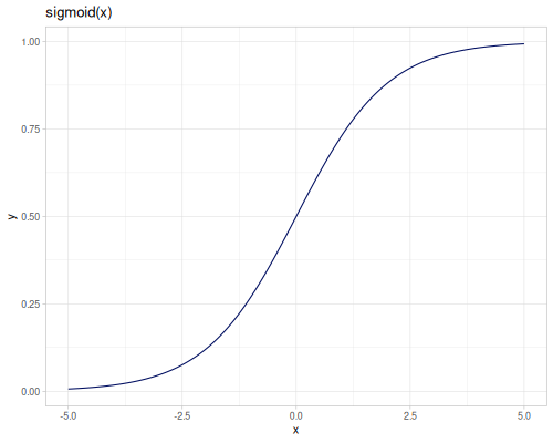
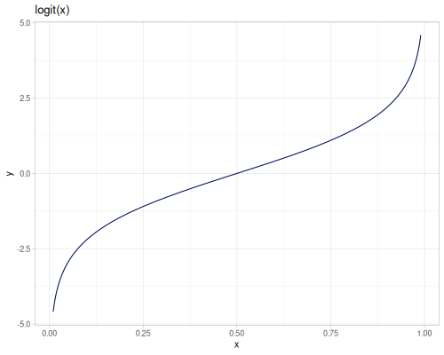
• sigmoid(x): Sigmoid function \(\sigma(x) = \frac{1}{1+e^{-x}}\). Also known as the logistic function.
• logit(x): Logit function \(\operatorname{logit}(x) = \ln(\frac{x}{1-x})\) for \(0 < x < 1\).

Examples

(m/sigmoid 0) ;; => 0.5
(m/sigmoid 10) ;; => 0.9999546021312976
(m/sigmoid -10) ;; => 4.5397868702434395E-5
(m/logit 0.5) ;; => 0.0
(m/logit 0.9) ;; => 2.1972245773362196
(m/logit 0.1) ;; => -2.197224577336219

Roots and Powers

Basic root and power functions.

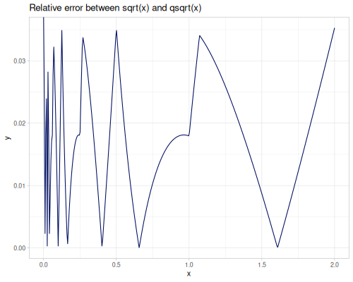
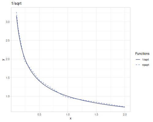
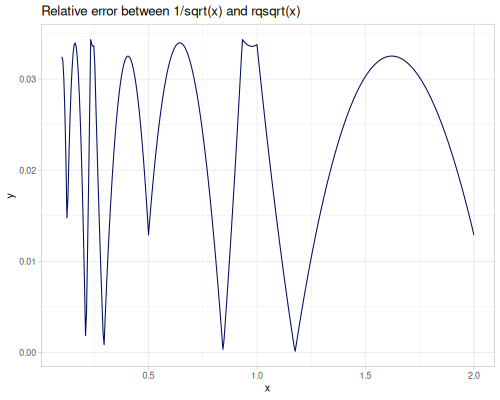
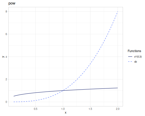
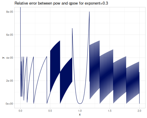
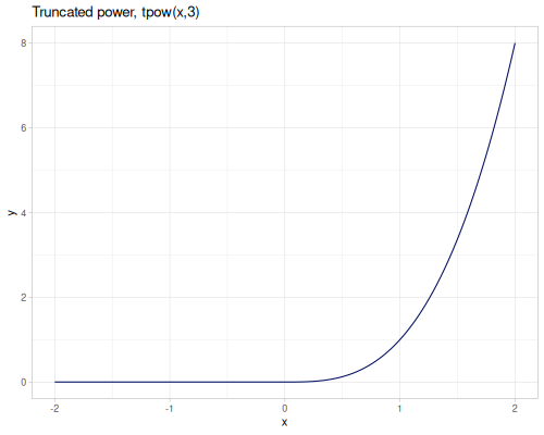
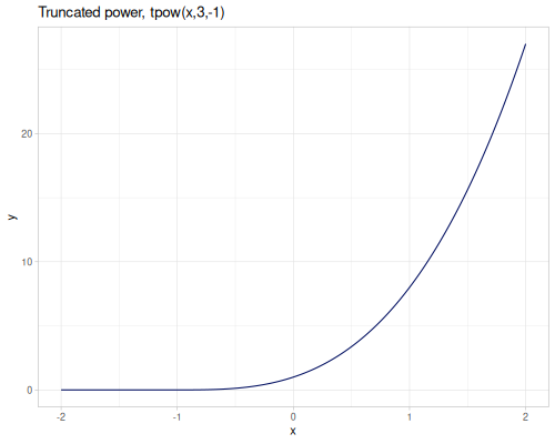
• sqrt(x): Square root \(\sqrt{x}\).
• cbrt(x): Cubic root \(\sqrt[3]{x}\).
• sq(x) or pow2(x): Square \(x^2\).
• cb(x) or pow3(x): Cube \(x^3\).
• pow10(x): \(x^{10}\).
• pow(x, exponent): \(x^{\text{exponent}}\).
• spow(x, exponent): Symmetric power of \(x\), keeping the sign: \(\operatorname{sgn}(x) |x|^{\text{exponent}}\).
• fpow(x, exponent): Fast integer power \(x^n\), where \(n\) is an integer.
• mpow(x, exponent, modulus): Modular exponentiation \(x^\text{exponent} \pmod{\text{modulus}}\).
• tpow(x, exponent, shift): Truncated power \((x-\text{shift})^\text{exponent}\) for \(x\ge \text{shift}\), \(0.0\) otherwise.
• qsqrt(x): Fast, less accurate square root.
• rqsqrt(x): Fast, less accurate reciprocal square root \(1/\sqrt{x}\).
• safe-sqrt(x): Square root, returning 0 for \(x \le 0\).

Examples

(m/sqrt 9) ;; => 3.0
(m/qsqrt 9) ;; => 3.053203231465716
(m/rqsqrt 9) ;; => 0.3424875211975356
(m/cbrt 27) ;; => 3.0
(m/sq 3) ;; => 9.0
(m/cb 3) ;; => 27.0
(m/pow 2 3) ;; => 8.0
(m/pow 9 0.5) ;; => 3.0
(m/pow 0.2 0.3) ;; => 0.6170338627200097
(m/qpow 0.2 0.3) ;; => 0.61701691483573
(m/spow -8 1/3) ;; => -2.0
(m/fpow 2 10) ;; => 1024.0
(m/mpow 30 112 74) ;; => 70
(m/tpow 3 3) ;; => 27.0
(m/tpow -3 3) ;; => 0.0
(m/tpow 6 3 2) ;; => 64.0
(m/tpow 0 3 2) ;; => 0.0
(m/safe-sqrt -4) ;; => 0.0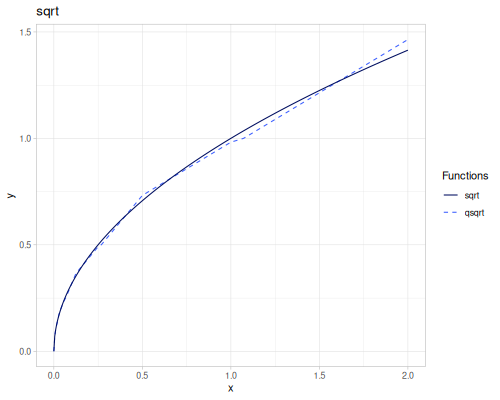

Exponent/Log Utilities

Functions related to powers of 2 and general bases.

• low-2-exp(x): Finds the largest integer \(n\) such that \(2^n \le |x|\). Returns long.
• high-2-exp(x): Finds the smallest integer \(n\) such that \(2^n \ge |x|\). Returns long.
• low-exp(b, x): Finds the largest integer \(n\) such that \(b^n \le |x|\). Returns long.
• high-exp(b, x): Finds the smallest integer \(n\) such that \(b^n \ge |x|\). Returns long.

Examples

(m/low-2-exp 10) ;; => 3
(m/high-2-exp 10) ;; => 4
(m/low-exp 10 150) ;; => 2
(m/high-exp 10 150) ;; => 3

Bitwise operations

Functions for performing bitwise operations on long primitive types.

Defined functions

• bit-and, bit-or, bit-xor,
• bit-not, bit-nand, bit-nor, bit-xnor, bit-and-not
• bit-set, bit-clear, bit-flip, bit-test
• <<, bit-shift-left, >>, bit-shift-right, >>>, unsigned-bit-shift-right

Logical Bitwise Operations

These functions perform standard logical operations on the individual bits of their long arguments. They are inlined and accept one or more arguments for multi-arity operations.

• bit-and: Bitwise AND (\(\land\)).
• bit-or: Bitwise OR (\(\lor\)).
• bit-xor: Bitwise XOR (\(\oplus\)).
• bit-not: Bitwise NOT (\(\sim\)).
• bit-nand: Bitwise NAND (\(\neg (x \land y)\)).
• bit-nor: Bitwise NOR (\(\neg (x \lor y)\)).
• bit-xnor: Bitwise XNOR (\(\neg (x \oplus y)\)).
• bit-and-not: Bitwise AND with complement of the second argument (\(x \land \sim y\)).

Examples

(m/bit-and 12 10) ;; => 8
(m/bit-or 12 10) ;; => 14
(m/bit-xor 12 10) ;; => 6
(m/bit-not 12) ;; => -13
(m/bit-nand 12 10) ;; => -9
(m/bit-nor 12 10) ;; => -15
(m/bit-xnor 12 10) ;; => -7
(m/bit-and-not 12 10) ;; => 4
(kind/md "Multi-arity examples") ;; => ["Multi-arity examples"]
(m/bit-and 15 12 10) ;; => 8
(m/bit-or 0 12 10) ;; => 14
(m/bit-xor 15 12 10) ;; => 9

Bit Shift Operations

These functions shift the bits of a long value left or right.

• << / bit-shift-left: Signed left shift (\(x \ll \text{shift}\)). Bits shifted off the left are discarded, and zero bits are shifted in from the right.
• >> / bit-shift-right: Signed right shift (\(x \gg \text{shift}\)). Bits shifted off the right are discarded. The sign bit (the leftmost bit) is extended to fill in from the left, preserving the number’s sign.
• >>> / unsigned-bit-shift-right: Unsigned right shift (\(x \ggg \text{shift}\)). Bits shifted off the right are discarded. Zero bits are shifted in from the left, regardless of the number’s sign.

Examples

(m/<< 12 2) ;; => 48
(m/bit-shift-left 12 2) ;; => 48
(m/>> 12 2) ;; => 3
(m/bit-shift-right 12 2) ;; => 3
(m/>> -12 2) ;; => -3
(m/bit-shift-right -12 2) ;; => -3
(m/>>> 12 2) ;; => 3
(m/unsigned-bit-shift-right 12 2) ;; => 3
(m/>>> -12 2) ;; => 4611686018427387901
(m/unsigned-bit-shift-right -12 2) ;; => 4611686018427387901

Bit Manipulation

Functions to manipulate individual bits within a long value.

• bit-set: Sets a specific bit at the given index to 1.
• bit-clear: Clears a specific bit at the given index to 0.
• bit-flip: Flips the state of a specific bit at the given index (0 becomes 1, 1 becomes 0).
• bit-test: Tests the state of a specific bit at the given index. Returns true if the bit is 1, false if it is 0.

Examples

(m/bit-set 10 1) ;; => 10
(m/bit-clear 10 3) ;; => 2
(m/bit-flip 10 2) ;; => 14
(m/bit-test 10 1) ;; => true
(m/bit-test 10 0) ;; => false

Floating point

Functions for inspecting and manipulating the binary representation of floating-point numbers, and for finding adjacent floating-point values.

Defined functions

• next-double, prev-double, ulp
• double-bits, double-high-bits, double-low-bits, bits->double
• double-exponent, double-significand

• next-double(x): Returns the floating-point value adjacent to x in the direction of positive infinity. Can take an optional delta argument to find the value delta steps away.
• prev-double(x): Returns the floating-point value adjacent to x in the direction of negative infinity. Can take an optional delta argument to find the value delta steps away.
• ulp(x): Returns the size of an ulp of x - the distance between this floating-point value and the floating-point value adjacent to it. Formally, it’s the spacing between floating-point numbers in the neighborhood of x.
• double-bits(x): Returns the 64-bit long integer representation of the double value x according to the IEEE 754 floating-point “double format” bit layout.
• double-high-bits(x): Returns the high 32 bits of the double value x’s IEEE 754 representation as a long.
• double-low-bits(x): Returns the low 32 bits of the double value x’s IEEE 754 representation as a long.
• bits->double(bits): Returns the double floating-point value corresponding to the given 64-bit long integer representation. This is the inverse of double-bits.
• double-exponent(x): Returns the unbiased exponent of the double value x.
• double-significand(x): Returns the significand (mantissa) of the double value x as a long. This is the 52 explicit bits of the significand for normalized numbers.
• log2int(x): Returns an integer approximation of \(\log_2(|x|)\). It’s closely related to double-exponent but includes an adjustment based on the significand to provide a more precise floor-like integer log.

Examples

(m/next-double 0.0) ;; => 4.9E-324
(m/next-double -0.0) ;; => 4.9E-324
(m/next-double 1.0) ;; => 1.0000000000000002
(m/next-double 1.0 10) ;; => 1.0000000000000022
(m/next-double 1.0E20) ;; => 1.0000000000000002E20
(m/prev-double 0.0) ;; => -4.9E-324
(m/prev-double 1.0) ;; => 0.9999999999999999
(m/prev-double 1.0 10) ;; => 0.9999999999999989
(m/prev-double 1.0E20) ;; => 9.999999999999998E19
(m/ulp 1.0) ;; => 2.220446049250313E-16
(m/ulp 2.0) ;; => 4.440892098500626E-16
(m/ulp 1.0E20) ;; => 16384.0
(m/log2int 8.0) ;; => 3
(m/double-exponent 8.0) ;; => 3
(m/log2int 7.1) ;; => 3
(m/double-exponent 7.1) ;; => 2

Now let’s convert 123.456 to internal representation.

(let [d 123.456] {:double d, :bits (m/double-bits d), :high (m/double-high-bits d), :low (m/double-low-bits d), :exponent (m/double-exponent d), :significand (m/double-significand d)})

{:bits 4638387860618067575,
 :double 123.456,
 :exponent 6,
 :high 1079958831,
 :low 446676599,
 :significand 4183844053827191}

Convert back to a double:

(m/bits->double 4638387860618067575)

123.45600000000559

Combinatorics

Functions for common combinatorial calculations, including factorials and binomial coefficients.

Defined functions

• factorial20, factorial, inv-factorial, log-factorial
• falling-factorial, falling-factorial-int, rising-factorial, rising-factorial-int
• combinations, log-combinations

Factorials

The factorial of a non-negative integer \(n\), denoted by \(n!\), is the product of all positive integers less than or equal to \(n\). \(0!\) is defined as \(1\).

• factorial20(n): Computes \(n!\) for \(0 \le n \le 20\) using a precomputed table. Returns long.
• factorial(n): Computes \(n!\) for any non-negative integer \(n\). For \(n > 20\), it uses the Gamma function: \(n! = \Gamma(n+1)\). Returns double.
• inv-factorial(n): Computes the inverse factorial, \(\frac{1}{n!}\). Returns double.
• log-factorial(n): Computes the natural logarithm of the factorial, \(\ln(n!) = \ln(\Gamma(n+1))\). Returns double.

Examples

(m/factorial 5) ;; => 120.0
(m/factorial20 5) ;; => 120
(m/factorial 21) ;; => 5.1090942171709776E19
(m/inv-factorial 5) ;; => 0.008333333333333333
(m/log-factorial 5) ;; => 4.787491742782046

Factorial-like products

These functions generalize the factorial to falling (descending) and rising (Pochhammer) products.

• falling-factorial-int(n, x): Computes the falling factorial \(x^{\underline{n}} = x(x-1)\dots(x-n+1)\) for integer \(n \ge 0\).
• falling-factorial(n, x): Computes the falling factorial for real \(n\), \(x^{\underline{n}} = \frac{\Gamma(x+1)}{\Gamma(x-n+1)}\).
• rising-factorial-int(n, x): Computes the rising factorial (Pochhammer symbol) \(x^{\overline{n}} = x(x+1)\dots(x+n-1)\) for integer \(n \ge 0\).
• rising-factorial(n, x): Computes the rising factorial for real \(n\), \(x^{\overline{n}} = \frac{\Gamma(x+n)}{\Gamma(x)}\).

Examples

(m/falling-factorial-int 3 10) ;; => 720.0
(m/falling-factorial 3.5 10.0) ;; => 1939.2340147230293
(m/rising-factorial-int 3 10) ;; => 1320.0
(m/rising-factorial 3.5 10.0) ;; => 4713.795382273956

Combinations

The binomial coefficient \(\binom{n}{k}\) represents the number of ways to choose \(k\) elements from a set of \(n\) distinct elements, without regard to the order of selection.

• combinations(n, k): Computes the binomial coefficient \(\binom{n}{k} = \frac{n!}{k!(n-k)!}\). Returns double.
• log-combinations(n, k): Computes the natural logarithm of the binomial coefficient, \(\ln\binom{n}{k}\). Returns double.

Examples

(m/combinations 10 2) ;; => 45.0
(m/combinations 10 8) ;; => 45.0
(m/combinations 5 0) ;; => 1.0
(m/combinations 5 6) ;; => 0.0
(m/log-combinations 10 2) ;; => 3.8066624897703196
(m/log-combinations 1000 500) ;; => 689.4672615678511

Rank and order

Functions for determining the rank of elements within a collection and the order (indices) required to sort it.

Defined functions

• rank, rank1
• order

rank computes the rank of each element in a collection. Ranks are 0-based indices indicating the position an element would have if the collection were sorted. It supports various tie-breaking strategies:

• :average: Assign the average rank to tied elements (default).
• :first: Assign ranks based on their original order for ties.
• :last: Assign ranks based on their original order (reverse of :first).
• :random: Assign random ranks for ties.
• :min: Assign the minimum rank to tied elements.
• :max: Assign the maximum rank to tied elements.
• :dense: Assign consecutive ranks without gaps for tied elements.

It also supports ascending (default) and descending order.

rank1 is identical to rank but returns 1-based indices.

(def data [5 1 8 1 5 1 1 1])

Examples

Ascending

(m/rank data) ;; => (5.5 2.0 7.0 2.0 5.5 2.0 2.0 2.0)
(m/rank data :dense) ;; => (1 0 2 0 1 0 0 0)
(m/rank data :min) ;; => (5 0 7 0 5 0 0 0)
(m/rank data :max) ;; => (6 4 7 4 6 4 4 4)
(m/rank data :random) ;; => [5 1 7 4 6 3 2 0]
(m/rank data :random) ;; => [6 2 7 3 5 0 4 1]
(m/rank data :first) ;; => [5 0 7 1 6 2 3 4]
(m/rank data :last) ;; => [6 4 7 3 5 2 1 0]

Descending

(m/rank data :average true) ;; => (1.5 5.0 0.0 5.0 1.5 5.0 5.0 5.0)
(m/rank data :dense true) ;; => (1 2 0 2 1 2 2 2)
(m/rank data :min true) ;; => (1 3 0 3 1 3 3 3)
(m/rank data :max true) ;; => (2 7 0 7 2 7 7 7)
(m/rank data :random true) ;; => [1 6 0 4 2 3 5 7]
(m/rank data :random true) ;; => [2 6 0 3 1 7 4 5]
(m/rank data :first true) ;; => [1 3 0 4 2 5 6 7]
(m/rank data :last true) ;; => [2 7 0 6 1 5 4 3]

1-based indices

(m/rank1 data) ;; => (6.5 3.0 8.0 3.0 6.5 3.0 3.0 3.0)

order computes the indices that would sort the collection. Applying these indices to the original collection yields the sorted sequence.

Examples

(m/order data) ;; => (1 3 5 6 7 0 4 2)
(map data (m/order data)) ;; => (1 1 1 1 1 5 5 8)
(m/order data true) ;; => (2 0 4 1 3 5 6 7)
(map data (m/order data true)) ;; => (8 5 5 1 1 1 1 1)

Interpolation and mapping

Functions for mapping values between numerical ranges (normalization) and for various types of interpolation, smoothing the transition between values. These tools are useful for graphics, animation, signal processing, and data manipulation.

Defined functions

• norm, mnorm, cnorm, make-norm
• lerp, mlerp
• smoothstep
• cos-interpolation, smooth-interpolation, quad-interpolation

Mapping and Normalization

These functions map a value from one numerical range to another.

• norm(v, start, stop): Maps v from the range \([start, stop]\) to \([0, 1]\). The formula is \(\frac{v - start}{stop - start}\).
• norm(v, start1, stop1, start2, stop2): Maps v from the range \([start1, stop1]\) to \([start2, stop2]\). The formula is \(start2 + (stop2 - start2) \frac{v - start1}{stop1 - start1}\).
• mnorm: Macro version of norm for inlining.
• cnorm: Constrained version of norm. The result is clamped to the target range \([0, 1]\) or \([start2, stop2]\).
• make-norm(start, stop, [dstart, dstop]): Creates a function that maps values from \([start, stop]\) to \([0, 1]\) or \([dstart, dstop]\).

Examples

(m/norm 5 0 10) ;; => 0.5
(m/norm 15 0 10) ;; => 1.5
(m/norm 5 0 10 100 200) ;; => 150.0
(m/cnorm 5 0 10) ;; => 0.5
(m/cnorm 15 0 10) ;; => 1.0
(m/cnorm -5 0 10 100 200) ;; => 100.0
(let [map-fn (m/make-norm 0 10 100 200)] (map-fn 5)) ;; => 150.0
(let [map-fn (m/make-norm 0 10)] (map-fn 5 100 200)) ;; => 150.0

Interpolation

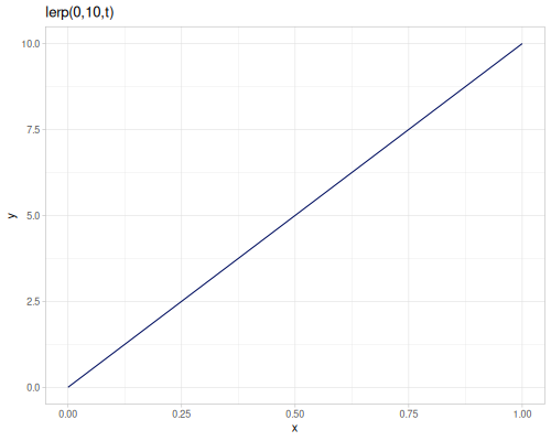
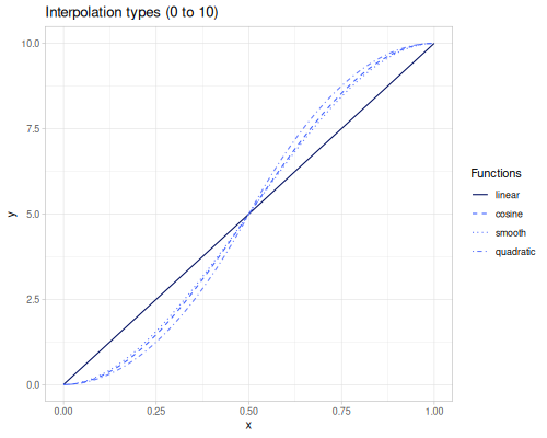
Interpolation functions find intermediate values between two points based on a blending factor, often called t (for time). The factor t typically ranges from 0 to 1, where t=0 corresponds to the start value and t=1 to the stop value.

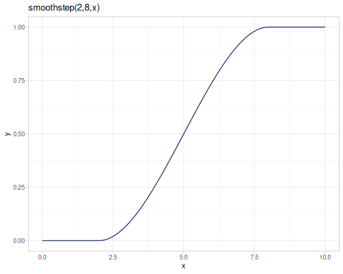
• lerp(start, stop, t): Linear interpolation. Blends start and stop linearly based on t. The formula is \(start + t \cdot (stop - start)\).
• mlerp: Macro version of lerp for inlining.
• smoothstep(edge0, edge1, x): Smooth interpolation between 0 and 1. If \(x \le edge0\), returns 0. If \(x \ge edge1\), returns 1. Otherwise, it performs a cubic Hermite interpolation for \(x\) mapped from \([edge0, edge1]\) to \([0, 1]\). This provides a smooth transition with zero derivative at the edges. The formula for the interpolation step is \(t^2 (3 - 2t)\), where \(t = \operatorname{cnorm}(x, edge0, edge1)\).
• cos-interpolation(start, stop, t): Cosine interpolation. Uses a cosine curve to smooth the transition between start and stop.
• smooth-interpolation(start, stop, t): Uses the smoothstep interpolation curve (cubic \(3t^2 - 2t^3\)) to blend start and stop.
• quad-interpolation(start, stop, t): Quadratic interpolation. Uses a parabolic curve, giving a faster initial and slower final rate of change compared to linear.

Examples

(m/lerp 0 10 0.5) ;; => 5.0
(m/lerp 0 10 0.0) ;; => 0.0
(m/lerp 0 10 1.0) ;; => 10.0
(m/smoothstep 2 8 1) ;; => 0.0
(m/smoothstep 2 8 5) ;; => 0.5
(m/smoothstep 2 8 9) ;; => 1.0
(m/cos-interpolation 0 10 0.5) ;; => 4.999999999999999
(m/smooth-interpolation 0 10 0.5) ;; => 5.0
(m/quad-interpolation 0 10 0.5) ;; => 5.0

Distance

Functions for calculating distances between points or the magnitude (Euclidean norm) of vectors, including specialized functions for geographic distances.

Defined functions

• dist, qdist, hypot, hypot-sqrt
• haversine-dist

• dist(x1, y1, x2, y2): Calculates the Euclidean distance between two 2D points \((x_1, y_1)\) and \((x_2, y_2)\). Also accepts pairs of coordinates [x1 y1] and [x2 y2]. \[ \operatorname{dist}((x_1, y_1), (x_2, y_2)) = \sqrt{(x_2 - x_1)^2 + (y_2 - y_1)^2} \]
• qdist: A faster, less accurate version of dist using [qsqrt] instead of [sqrt].
• hypot(x, y) and hypot(x, y, z): Calculates the Euclidean norm (distance from the origin) of a 2D or 3D vector \(\sqrt{x^2 + y^2}\) or \(\sqrt{x^2 + y^2 + z^2}\). This function uses a numerically stable algorithm to avoid potential overflow or underflow issues compared to a direct calculation. \[ \operatorname{hypot}(x, y) = \sqrt{x^2 + y^2} \] \[ \operatorname{hypot}(x, y, z) = \sqrt{x^2 + y^2 + z^2} \]
• hypot-sqrt(x, y) and hypot-sqrt(x, y, z): Calculates the Euclidean norm using the direct formula \(\sqrt{x^2+y^2}\) or \(\sqrt{x^2+y^2+z^2}\). This may be less numerically stable than [hypot] for inputs with vastly different magnitudes.
• haversine-dist(lat1, lon1, lat2, lon2): Calculates the great-circle distance between two points on a sphere given their latitude and longitude (in radians), assuming a sphere with radius \(R=1\). This function uses the haversine formula component computed by [haversin] (described in the Trigonometry section) and the inverse haversine formula to find the angle, then scales by \(R=1\). Also accepts coordinate pairs [lat1 lon1] and [lat2 lon2]. The distance is \(d = 2 \arcsin(\sqrt{a})\), where \(a\) is the value computed by (haversin lat1 lon1 lat2 lon2).

Examples

(m/dist 0 0 3 4) ;; => 5.0
(m/dist [0 0] [3 4]) ;; => 5.0
(m/qdist 0 0 3 4) ;; => 4.981406462931432
(m/hypot 3 4) ;; => 5.0
(m/hypot 1.0E150 1.0E250) ;; => 1.0E250
(m/hypot-sqrt 1.0E150 1.0E250) ;; => ##Inf
(m/hypot 2 3 4) ;; => 5.385164807134504
(m/haversine-dist (m/radians 38.898) (m/radians 77.037) (m/radians 48.858) (m/radians -2.294)) ;; => 0.9671068960642187
(m/haversine-dist [(m/radians 38.898) (m/radians 77.037)] [(m/radians 48.858) (m/radians -2.294)]) ;; => 0.9671068960642187

Intervals

Functions for partitioning numerical ranges and grouping data into intervals. These are useful for data analysis, histogram creation, and data binning.

Defined functions

• slice-range, cut
• co-intervals, group-by-intervals
• sample

• slice-range(cnt) / slice-range(start, end, cnt): Generates a sequence of cnt evenly spaced double values between start and end (inclusive). If only cnt is provided, the range [0.0, 1.0] is used. If cnt is 1, returns the midpoint.
• cut(data, breaks) / cut(x1, x2, breaks): Divides a numerical range into breaks adjacent intervals. The range is either explicitly given by x1, x2 or determined by the min/max finite values in data. Returns a sequence of 2-element vectors [lower-bound upper-bound]. The intervals are effectively \([min\_value, p_1], (p_1, p_2], \dots, (p_{breaks-1}, max\_value]\). The lower bound of the first interval is slightly adjusted downwards using [prev-double] to ensure the exact minimum is included.

Examples

(m/slice-range 5) ;; => (0.0 0.25 0.5 0.75 1.0)
(m/slice-range -10 10 5) ;; => (-10.0 -5.0 0.0 5.0 10.0)
(m/cut (range 10) 3) ;; => ((-4.9E-324 3.0) (3.0 6.0) (6.0 9.0))
(m/cut 0 9 3) ;; => ((-4.9E-324 3.0) (3.0 6.0) (6.0 9.0))

• co-intervals(data, [number, overlap]): Generates number (default 6) overlapping intervals from the sorted finite values in data. Each interval aims to contain a similar number of data points. overlap (default 0.5) controls the proportion of overlap between consecutive intervals. Returns a sequence of 2-element vectors [lower-bound upper-bound].
• group-by-intervals(intervals, coll) / group-by-intervals(coll): Groups the values in coll into the provided intervals. Returns a map where keys are the interval vectors and values are sequences of numbers from coll falling into that interval (checked using [between-?] for \((lower, upper]\)). If no intervals are provided, it first computes them using [co-intervals] on coll.

(def sample-data (repeatedly 20 #(+ (rand 10) (rand 10) (rand 10))))

Examples

(m/co-intervals sample-data 4) ;; => ([4.87954821907383 12.612957116093272] [8.039881226728655 13.411937120554235] [12.635320112604235 16.884612368709163] [13.860329720205982 23.58863731178268])
(m/co-intervals sample-data 4 0.2) ;; => ([4.87954821907383 10.606717713515938] [10.59924157536398 13.274199400788818] [12.81667190852161 16.877136230557205] [16.869660092405248 23.58863731178268])

(into (sorted-map) (m/group-by-intervals (m/co-intervals sample-data 4) sample-data))

{[12.635320112604235 16.884612368709163] (16.873398161481227
                                          13.864067789281961
                                          12.639058181680214
                                          16.880874299633184
                                          13.408199051478256
                                          15.21133109212528
                                          12.820409977597588
                                          13.27046133171284),
 [13.860329720205982 23.58863731178268] (16.873398161481227
                                         13.864067789281961
                                         23.5848992427067
                                         19.0503381374082
                                         16.880874299633184
                                         18.219530772828655
                                         15.21133109212528
                                         22.659747743467783),
 [4.87954821907383 12.612957116093272] (10.602979644439959
                                        8.043619295804634
                                        5.051463038340989
                                        4.883286288149809
                                        7.265862554091448
                                        10.798056102722585
                                        7.399126826393544
                                        12.609219047017293),
 [8.039881226728655 13.411937120554235] (10.602979644439959
                                         8.043619295804634
                                         12.639058181680214
                                         13.408199051478256
                                         12.820409977597588
                                         10.798056102722585
                                         13.27046133171284
                                         12.609219047017293)}

Function sampling

sample(f, number-of-values, [domain-min, domain-max, domain?]): Samples a function f by evaluating it at number-of-values evenly spaced points within the specified [domain-min, domain-max] range. If domain? is true, returns [x, (f x)] pairs; otherwise, returns just (f x) values. Defaults to sampling 6 values in the [0, 1] range.

Examples

(m/sample m/sin 0 m/PI 5) ;; => (0.0 0.7071067811865475 1.0 0.7071067811865477 1.224646799076922E-16)
(m/sample m/sin 0 m/PI 5 true) ;; => ([0.0 0.0] [0.7853981633974483 0.7071067811865475] [1.5707963267948966 1.0] [2.356194490192345 0.7071067811865477] [3.141592653589793 1.224646799076922E-16])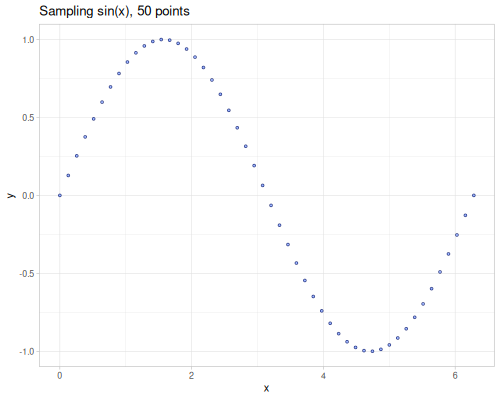

Other

This section contains a collection of miscellaneous utility functions that don’t fit neatly into the preceding categories, including integer number theory functions, boolean operations, data structure conversions, and error calculation utilities.

Defined functions

• gcd, lcm
• bool-not, bool-xor, xor
• identity-long, identity-double
• relative-error, absolute-error
• seq->double-array, seq->double-double-array, double-array->seq, double-double-array->seq
• use-primitive-operators, unuse-primitive-operators

Number Theory

Functions for calculating the greatest common divisor (GCD) and least common multiple (LCM) of integers.

• gcd(a, b): Computes the greatest common divisor of two long integers a and b. Uses the binary GCD algorithm (Stein’s algorithm), which is typically faster than the Euclidean algorithm for integers. \[ \operatorname{gcd}(a, b) = \max \{ d \in \mathbb{Z}^+ : d \mid a \land d \mid b \} \]
• lcm(a, b): Computes the least common multiple of two long integers a and b. \[ \operatorname{lcm}(a, b) = \frac{|a \cdot b|}{\operatorname{gcd}(a, b)} \]

Examples

(m/gcd 12 18) ;; => 6
(m/gcd 35 49) ;; => 7
(m/gcd 17 23) ;; => 1
(m/lcm 12 18) ;; => 36
(m/lcm 35 49) ;; => 245
(m/lcm 17 23) ;; => 391

Boolean and Identity Utilities

Basic boolean operations and identity functions for primitive types.

• bool-not(x): Primitive boolean NOT. Returns true if x is logically false, false otherwise.
• bool-xor(x, y) / xor(x, y): Primitive boolean XOR (exclusive OR). Returns true if exactly one of x or y is logically true. Accepts multiple arguments, chaining the XOR operation.
• identity-long(x): Returns its long argument unchanged. Useful for type hinting or guaranteeing a long primitive.
• identity-double(x): Returns its double argument unchanged. Useful for type hinting or guaranteeing a double primitive.

Examples

(m/bool-not true) ;; => false
(m/bool-not false) ;; => true
(m/xor true false) ;; => true
(m/xor true true) ;; => false
(m/xor true false true) ;; => false
(m/identity-long 5) ;; => 5
(m/identity-double 5.0) ;; => 5.0

Error Calculation

Functions to compute the difference between a value and its approximation.

• absolute-error(v, v-approx): Computes the absolute difference between a value v and its approximation v-approx. \[ \operatorname{absolute-error}(v, v_{\text{approx}}) = |v - v_{\text{approx}}| \]
• relative-error(v, v-approx): Computes the relative difference between a value v and its approximation v-approx. \[ \operatorname{relative-error}(v, v_{\text{approx}}) = \left| \frac{v - v_{\text{approx}}}{v} \right| \]

Examples

(m/absolute-error 10.0 10.01) ;; => 0.009999999999999787
(m/relative-error 10.0 10.01) ;; => 9.999999999999788E-4
(m/absolute-error 1.0E-6 1.01E-6) ;; => 1.0000000000000116E-8
(m/relative-error 1.0E-6 1.01E-6) ;; => 0.010000000000000116

Array and Sequence Conversion

Utilities for converting between Clojure sequences and primitive Java arrays (double[] and double[][]). These are often necessary for interoperation with Java libraries or for performance-critical operations.

• seq->double-array(vs): Converts a sequence vs into a double[] array. If vs is already a double[], it is returned directly. If vs is a single number, returns a double[] of size 1 containing that number.
• double-array->seq(res): Converts a double[] array res into a sequence. This is an alias for Clojure’s built-in seq function which works correctly for Java arrays.
• seq->double-double-array(vss): Converts a sequence of sequences vss into a double[][] array. If vss is already a double[][], it is returned directly.
• double-double-array->seq(res): Converts a double[][] array res into a sequence of sequences.

Examples

(m/seq->double-array [1 2 3]) ;; => #object["[D" 0x75b13441 "[D@75b13441"]
(m/double-array->seq (double-array [1.0 2.0 3.0])) ;; => (1.0 2.0 3.0)
(m/seq->double-double-array [[1 2] [3 4]]) ;; => #object["[[D" 0x3978890d "[[D@3978890d"]
(m/double-double-array->seq (into-array (map double-array [[1 2] [3 4]]))) ;; => ((1.0 2.0) (3.0 4.0))

Primitive Operators Toggle

Macros to replace or restore core Clojure math functions with fastmath.core primitive-specialized versions. This can improve performance but should be used carefully as the fastmath.core versions have specific type and return value behaviors.

• use-primitive-operators: Replaces a select set of clojure.core functions (like +, -, *, /, comparison operators, bitwise operators, inc, dec, predicates) with their primitive-specialized fastmath.core macro equivalents within the current namespace.
• unuse-primitive-operators: Reverts the changes made by use-primitive-operators, restoring the original clojure.core functions in the current namespace. Recommended practice is to call this at the end of any namespace that calls use-primitive-operators (especially important in Clojure 1.12+).

Example usage (typically done at the top or bottom of a namespace):

(ns my-namespace (:require [fastmath.core :as m]))
(m/use-primitive-operators)
... your code using primitive math ...
(m/unuse-primitive-operators) ;; or at the end of the file

Constants

Constant symbol	Value	Description
-E	-2.718281828459045	Value of \(-\mathrm{e}\)
-HALF_PI	-1.5707963267948966	Value of \(\frac{\pi}{2}\)
-PI	-3.141592653589793	Value of \(-\pi\)
-QUARTER_PI	-0.7853981633974483	Value of \(\frac{\pi}{4}\)
-TAU	-6.283185307179586	Value of \(-2\pi\)
-THIRD_PI	1.0471975511965976	Value of \(\frac{\pi}{3}\)
-TWO_PI	-6.283185307179586	Value of \(-2\pi\)
CATALAN_G	0.915965594177219	Catalan G
E	2.718281828459045	Value of \(\mathrm{e}\)
EPSILON	1.0E-10	\(\varepsilon\), a small number
FOUR_INV_PI	1.2732395447351628	Value of \(\frac{4}{\pi}\)
GAMMA	0.5772156649015329	\(\gamma\), Euler-Mascheroni constant
HALF_PI	1.5707963267948966	Value of \(\frac{\pi}{2}\)
INV_FOUR_PI	0.07957747154594767	Value of \(\frac{2}{2\pi}\)
INV_LN2	1.4426950408889634	Value of \(\frac{1}{\ln{2}}\)
INV_LOG_HALF	-1.4426950408889634	Value of \(\frac{1}{\ln{\frac{1}{2}}}\)
INV_PI	0.3183098861837907	Value of \(\frac{1}{\pi}\)
INV_SQRT2PI	0.3989422804014327	Value of \(\frac{1}{\sqrt{2\pi}}\)
INV_SQRTPI	0.5641895835477563	Value of \(\frac{1}{\sqrt\pi}\)
INV_SQRT_2	0.7071067811865475	Value of \(\frac{1}{\sqrt{2}}\)
INV_TWO_PI	0.15915494309189535	Value of \(\frac{1}{2\pi}\)
LANCZOS_G	4.7421875	Lanchos approximation of g constant
LN10	2.302585092994046	Value of \(\ln{10}\)
LN2	0.6931471805599453	Value of \(\ln{2}\)
LN2_2	0.34657359027997264	Value of \(\frac{\ln{2}}{2}\)
LOG10E	0.4342944819032518	\(\log_{10}{\mathrm{e}}\)
LOG2E	1.4426950408889634	\(\log_{2}{\mathrm{e}}\)
LOG_HALF	-0.6931471805599453	Value of \(\ln{\frac{1}{2}}\)
LOG_PI	1.1447298858494002	Value of \(\ln{\pi}\)
LOG_TWO_PI	1.8378770664093453	Value of \(\ln{2\pi}\)
MACHINE-EPSILON	1.1102230246251565E-16	ulp(1)/2
MACHINE-EPSILON10	1.1102230246251565E-15	5ulp(1)
M_1_PI	0.3183098861837907	Value of \(\frac{1}{\pi}\)
M_2_PI	0.6366197723675814	Value of \(\frac{2}{\pi}\)
M_2_SQRTPI	1.1283791670955126	Value of \(\frac{2}{\sqrt\pi}\)
M_3PI_4	2.356194490192345	Value of \(\frac{3\pi}{4}\)
M_E	2.718281828459045	Value of \(\mathrm{e}\)
M_INVLN2	1.4426950408889634	Value of \(\frac{1}{\ln{2}}\)
M_IVLN10	0.43429448190325176	Value of \(\frac{1}{\ln{10}}\)
M_LN10	2.302585092994046	Value of \(\ln{10}\)
M_LN2	0.6931471805599453	Value of \(\ln{2}\)
M_LOG10E	0.4342944819032518	Value of \(\log_{10}{e}\)
M_LOG2E	1.4426950408889634	Value of \(\log_{2}{e}\)
M_LOG2_E	0.6931471805599453	Value of \(\ln{2}\)
M_PI	3.141592653589793	Value of \(\pi\)
M_PI_2	1.5707963267948966	Value of \(\frac{\pi}{2}\)
M_PI_4	0.7853981633974483	Value of \(\frac{\pi}{4}\)
M_SQRT1_2	0.7071067811865475	Value of \(\frac{1}{\sqrt{2}}\)
M_SQRT2	1.4142135623730951	Value of \(\sqrt{2}\)
M_SQRT3	1.7320508075688772	Value of \(\sqrt{3}\)
M_SQRT_PI	1.7724538509055159	Value of \(\sqrt\pi\)
M_TWOPI	6.283185307179586	Value of \(2\pi\)
ONE_SIXTH	0.16666666666666666	Value of \(\frac{1}{6}\)
ONE_THIRD	0.3333333333333333	Value of \(\frac{1}{3}\)
PHI	1.618033988749895	Golden ratio \(\phi\)
PI	3.141592653589793	Value of \(\pi\)
QUARTER_PI	0.7853981633974483	Value of \(\frac{\pi}{4}\)
SILVER	2.414213562373095	Silver ratio \(\delta_S\)
SIXTH	0.16666666666666666	Value of \(\frac{1}{6}\)
SQRT2	1.4142135623730951	Value of \(\sqrt{2}\)
SQRT2PI	2.5066282746310002	Value of \(\sqrt{2\pi}\)
SQRT2_2	0.7071067811865476	Value of \(\frac{\sqrt{2}}{2}\)
SQRT3	1.7320508075688772	Value of \(\sqrt{3}\)
SQRT3_2	0.8660254037844386	Value of \(\frac{\sqrt{3}}{2}\)
SQRT3_3	0.5773502691896257	Value of \(\frac{\sqrt{3}}{3}\)
SQRT3_4	0.4330127018922193	Value of \(\frac{\sqrt{3}}{4}\)
SQRT5	2.23606797749979	Value of \(\sqrt{5}\)
SQRTPI	1.7724538509055159	Value of \(\sqrt{\pi}\)
SQRT_2_PI	0.7978845608028654	Value of \(\sqrt{\frac{2}{\pi}}\)
SQRT_HALFPI	1.2533141373155001	Value of \(\sqrt{\frac{1}{2}\pi}\)
TAU	6.283185307179586	Value of \(2\pi\)
THIRD	0.3333333333333333	Value of \(\frac{1}{3}\)
THIRD_PI	1.0471975511965976	Value of \(\frac{\pi}{3}\)
TWO_INV_PI	0.6366197723675814	Value of \(\frac{2}{\pi}\)
TWO_PI	6.283185307179586	Value of \(2\pi\)
TWO_THIRD	0.6666666666666666	Value of \(\frac{2}{3}\)
TWO_THIRDS	0.6666666666666666	Value of \(\frac{2}{3}\)
deg-in-rad	0.017453292519943295	\(\frac{\pi}{180}\)
double-one-minus-epsilon	0.9999999999999999	Value of 0x1.fffffffffffffp-1d = 0.(9)
rad-in-deg	57.29577951308232	\(\frac{180}{\pi}\)

Reference

fastmath.core

High-performance mathematical functions and constants for Clojure, optimized for primitive double and long types.

Key features:

• Most functions are specialized for primitive types (double and long) and are inlined for performance.
• Primarily backed by the FastMath library and custom primitive implementations.
• Provides an option to replace clojure.core’s standard numerical operators with primitive-specialized macros.

This namespace contains functions for:

• Basic arithmetic (+, -, *, /, etc.)
• Comparisons and predicates (==, <, zero?, pos?, etc.)
• Bitwise operations
• Trigonometric and hyperbolic functions
• Exponents, logarithms, and powers
• Floating-point specific operations (ulp, bits manipulation)
• Combinatorics (factorial, combinations)
• Distance calculations
• Interpolation and mapping
• Utility functions (gcd, lcm, error calculation, etc.)

Primitive Math Operators:

A set of inlined macros designed to replace selected clojure.core arithmetic, comparison, and bitwise operators for potential performance gains with primitive arguments. These macros operate on double and long primitives and generally return primitive values.

Replaced operators:

• * + - / > < >= <= == rem quot mod
• bit-or bit-and bit-xor bit-not bit-and-not
• bit-shift-left bit-shift-right unsigned-bit-shift-right
• bit-set bit-clear bit-flip bit-test
• inc dec
• zero? neg? pos? even? odd?
• min max
• abs
• Additionally: << >> >>> not==

To enable these primitive operators in your namespace, call use-primitive-operators. To revert to the original clojure.core functions, call unuse-primitive-operators. Note that the fastmath.core versions are not a complete drop-in replacement due to their primitive-specific behavior (e.g., return types), and calling unuse-primitive-operators at the end of the namespace is recommended, especially in Clojure 1.12+.

*

• (*)
• (* a)
• (* a b)
• (* a b c)
• (* a b c d)
• (* a b c d & r)

Primitive and inlined *.

source

---

+

• (+)
• (+ a)
• (+ a b)
• (+ a b c)
• (+ a b c d)
• (+ a b c d & r)

Primitive and inlined +.

source

---

-

• (- a)
• (- a b)
• (- a b c)
• (- a b c d)
• (- a b c d & r)

Primitive and inlined -.

source

---

-E ^_CONST

-E = -2.718281828459045

Value of \(-\mathrm{e}\)

source

---

-HALF_PI ^_CONST

-HALF_PI = -1.5707963267948966

Value of \(\frac{\pi}{2}\)

source

---

-PI ^_CONST

-PI = -3.141592653589793

Value of \(-\pi\)

source

---

-QUARTER_PI ^_CONST

-QUARTER_PI = -0.7853981633974483

Value of \(\frac{\pi}{4}\)

source

---

-TAU ^_CONST

-TAU = -6.283185307179586

Value of \(-2\pi\)

source

---

-THIRD_PI ^_CONST

-THIRD_PI = 1.0471975511965976

Value of \(\frac{\pi}{3}\)

source

---

-TWO_PI ^_CONST

-TWO_PI = -6.283185307179586

Value of \(-2\pi\)

source

---

/

• (/ a)
• (/ a b)
• (/ a b c)
• (/ a b c d)
• (/ a b c d & r)

Primitive and inlined /.

source

---

<

• (< _)
• (< a b)
• (< a b & r)

Primitive math less-then function.

source

---

<<

• (<< x shift)

Shift bits left

source

---

<=

• (<= _)
• (<= a b)
• (<= a b & r)

Primitive math less-and-equal function.

source

---

==

• (== _)
• (== a b)
• (== a b & r)

Primitive math equality function.

source

---

>

• (> _)
• (> a b)
• (> a b & r)

Primitive math greater-than function.

source

---

>=

• (>= _)
• (>= a b)
• (>= a b & r)

Primitive math greater-and-equal function.

source

---

>>

• (>> x shift)

Shift bits right and keep most significant bit unchanged

source

---

>>>

• (>>> x shift)

Shift bits right and set most significant bit to 0

source

---

CATALAN_G ^_CONST

CATALAN_G = 0.915965594177219

Catalan G

source

---

E ^_CONST

E = 2.718281828459045

Value of \(\mathrm{e}\)

source

---

EPSILON ^_CONST

EPSILON = 1.0E-10

\(\varepsilon\), a small number

source

---

FOUR_INV_PI ^_CONST

FOUR_INV_PI = 1.2732395447351628

Value of \(\frac{4}{\pi}\)

source

---

GAMMA ^_CONST

GAMMA = 0.5772156649015329

\(\gamma\), Euler-Mascheroni constant

source

---

HALF_PI ^_CONST

HALF_PI = 1.5707963267948966

Value of \(\frac{\pi}{2}\)

source

---

INV_FOUR_PI ^_CONST

INV_FOUR_PI = 0.07957747154594767

Value of \(\frac{2}{2\pi}\)

source

---

INV_LN2 ^_CONST

INV_LN2 = 1.4426950408889634

Value of \(\frac{1}{\ln{2}}\)

source

---

INV_LOG_HALF ^_CONST

INV_LOG_HALF = -1.4426950408889634

Value of \(\frac{1}{\ln{\frac{1}{2}}}\)

source

---

INV_PI ^_CONST

INV_PI = 0.3183098861837907

Value of \(\frac{1}{\pi}\)

source

---

INV_SQRT2PI ^_CONST

INV_SQRT2PI = 0.3989422804014327

Value of \(\frac{1}{\sqrt{2\pi}}\)

source

---

INV_SQRTPI ^_CONST

INV_SQRTPI = 0.5641895835477563

Value of \(\frac{1}{\sqrt\pi}\)

source

---

INV_SQRT_2 ^_CONST

INV_SQRT_2 = 0.7071067811865475

Value of \(\frac{1}{\sqrt{2}}\)

source

---

INV_TWO_PI ^_CONST

INV_TWO_PI = 0.15915494309189535

Value of \(\frac{1}{2\pi}\)

source

---

LANCZOS_G ^_CONST

LANCZOS_G = 4.7421875

Lanchos approximation of g constant

source

---

LN10 ^_CONST

LN10 = 2.302585092994046

Value of \(\ln{10}\)

source

---

LN2 ^_CONST

LN2 = 0.6931471805599453

Value of \(\ln{2}\)

source

---

LN2_2 ^_CONST

LN2_2 = 0.34657359027997264

Value of \(\frac{\ln{2}}{2}\)

source

---

LOG10E ^_CONST

LOG10E = 0.4342944819032518

\(\log_{10}{\mathrm{e}}\)

source

---

LOG2E ^_CONST

LOG2E = 1.4426950408889634

\(\log_{2}{\mathrm{e}}\)

source

---

LOG_HALF ^_CONST

LOG_HALF = -0.6931471805599453

Value of \(\ln{\frac{1}{2}}\)

source

---

LOG_PI ^_CONST

LOG_PI = 1.1447298858494002

Value of \(\ln{\pi}\)

source

---

LOG_TWO_PI ^_CONST

LOG_TWO_PI = 1.8378770664093453

Value of \(\ln{2\pi}\)

source

---

MACHINE-EPSILON ^_CONST

MACHINE-EPSILON = 1.1102230246251565E-16

ulp(1)/2

source

---

MACHINE-EPSILON10 ^_CONST

MACHINE-EPSILON10 = 1.1102230246251565E-15

5ulp(1)

source

---

M_1_PI ^_CONST

M_1_PI = 0.3183098861837907

Value of \(\frac{1}{\pi}\)

source

---

M_2_PI ^_CONST

M_2_PI = 0.6366197723675814

Value of \(\frac{2}{\pi}\)

source

---

M_2_SQRTPI ^_CONST

M_2_SQRTPI = 1.1283791670955126

Value of \(\frac{2}{\sqrt\pi}\)

source

---

M_3PI_4 ^_CONST

M_3PI_4 = 2.356194490192345

Value of \(\frac{3\pi}{4}\)

source

---

M_E ^_CONST

M_E = 2.718281828459045

Value of \(\mathrm{e}\)

source

---

M_INVLN2 ^_CONST

M_INVLN2 = 1.4426950408889634

Value of \(\frac{1}{\ln{2}}\)

source

---

M_IVLN10 ^_CONST

M_IVLN10 = 0.43429448190325176

Value of \(\frac{1}{\ln{10}}\)

source

---

M_LN10 ^_CONST

M_LN10 = 2.302585092994046

Value of \(\ln{10}\)

source

---

M_LN2 ^_CONST

M_LN2 = 0.6931471805599453

Value of \(\ln{2}\)

source

---

M_LOG10E ^_CONST

M_LOG10E = 0.4342944819032518

Value of \(\log_{10}{e}\)

source

---

M_LOG2E ^_CONST

M_LOG2E = 1.4426950408889634

Value of \(\log_{2}{e}\)

source

---

M_LOG2_E ^_CONST

M_LOG2_E = 0.6931471805599453

Value of \(\ln{2}\)

source

---

M_PI ^_CONST

M_PI = 3.141592653589793

Value of \(\pi\)

source

---

M_PI_2 ^_CONST

M_PI_2 = 1.5707963267948966

Value of \(\frac{\pi}{2}\)

source

---

M_PI_4 ^_CONST

M_PI_4 = 0.7853981633974483

Value of \(\frac{\pi}{4}\)

source

---

M_SQRT1_2 ^_CONST

M_SQRT1_2 = 0.7071067811865475

Value of \(\frac{1}{\sqrt{2}}\)

source

---

M_SQRT2 ^_CONST

M_SQRT2 = 1.4142135623730951

Value of \(\sqrt{2}\)

source

---

M_SQRT3 ^_CONST

M_SQRT3 = 1.7320508075688772

Value of \(\sqrt{3}\)

source

---

M_SQRT_PI ^_CONST

M_SQRT_PI = 1.7724538509055159

Value of \(\sqrt\pi\)

source

---

M_TWOPI ^_CONST

M_TWOPI = 6.283185307179586

Value of \(2\pi\)

source

---

ONE_SIXTH ^_CONST

ONE_SIXTH = 0.16666666666666666

Value of \(\frac{1}{6}\)

source

---

ONE_THIRD ^_CONST

ONE_THIRD = 0.3333333333333333

Value of \(\frac{1}{3}\)

source

---

PHI ^_CONST

PHI = 1.618033988749895

Golden ratio \(\phi\)

source

---

PI ^_CONST

PI = 3.141592653589793

Value of \(\pi\)

source

---

QUARTER_PI ^_CONST

QUARTER_PI = 0.7853981633974483

Value of \(\frac{\pi}{4}\)

source

---

SILVER ^_CONST

SILVER = 2.414213562373095

Silver ratio \(\delta_S\)

source

---

SIXTH ^_CONST

SIXTH = 0.16666666666666666

Value of \(\frac{1}{6}\)

source

---

SQRT2 ^_CONST

SQRT2 = 1.4142135623730951

Value of \(\sqrt{2}\)

source

---

SQRT2PI ^_CONST

SQRT2PI = 2.5066282746310002

Value of \(\sqrt{2\pi}\)

source

---

SQRT2_2 ^_CONST

SQRT2_2 = 0.7071067811865476

Value of \(\frac{\sqrt{2}}{2}\)

source

---

SQRT3 ^_CONST

SQRT3 = 1.7320508075688772

Value of \(\sqrt{3}\)

source

---

SQRT3_2 ^_CONST

SQRT3_2 = 0.8660254037844386

Value of \(\frac{\sqrt{3}}{2}\)

source

---

SQRT3_3 ^_CONST

SQRT3_3 = 0.5773502691896257

Value of \(\frac{\sqrt{3}}{3}\)

source

---

SQRT3_4 ^_CONST

SQRT3_4 = 0.4330127018922193

Value of \(\frac{\sqrt{3}}{4}\)

source

---

SQRT5 ^_CONST

SQRT5 = 2.23606797749979

Value of \(\sqrt{5}\)

source

---

SQRTPI ^_CONST

SQRTPI = 1.7724538509055159

Value of \(\sqrt{\pi}\)

source

---

SQRT_2_PI ^_CONST

SQRT_2_PI = 0.7978845608028654

Value of \(\sqrt{\frac{2}{\pi}}\)

source

---

SQRT_HALFPI ^_CONST

SQRT_HALFPI = 1.2533141373155001

Value of \(\sqrt{\frac{1}{2}\pi}\)

source

---

TAU ^_CONST

TAU = 6.283185307179586

Value of \(2\pi\)

source

---

THIRD ^_CONST

THIRD = 0.3333333333333333

Value of \(\frac{1}{3}\)

source

---

THIRD_PI ^_CONST

THIRD_PI = 1.0471975511965976

Value of \(\frac{\pi}{3}\)

source

---

TWO_INV_PI ^_CONST

TWO_INV_PI = 0.6366197723675814

Value of \(\frac{2}{\pi}\)

source

---

TWO_PI ^_CONST

TWO_PI = 6.283185307179586

Value of \(2\pi\)

source

---

TWO_THIRD ^_CONST

TWO_THIRD = 0.6666666666666666

Value of \(\frac{2}{3}\)

source

---

TWO_THIRDS ^_CONST

TWO_THIRDS = 0.6666666666666666

Value of \(\frac{2}{3}\)

source

---

abs

• (abs x)

Absolute value.

source

---

absolute-error

• (absolute-error v v-approx)

Absolute error between two values

source

---

acos

• (acos x)

acos(x)

source

---

acosh

• (acosh x)

acosh(x)

source

---

acot

• (acot x)

acot(x)

source

---

acoth

• (acoth x)

Area hyperbolic cotangent

source

---

acovercos

• (acovercos x)

Arc covercosine

source

---

acoversin

• (acoversin x)

Arc coversine

source

---

acrd

• (acrd x)

Inverse chord

source

---

acsc

• (acsc x)

acsc(x)

source

---

acsch

• (acsch v)

Area hyperbolic cosecant

source

---

aexcsc

• (aexcsc x)

Arc excosecant

source

---

aexsec

• (aexsec x)

Arc exsecant

source

---

ahacovercos

• (ahacovercos x)

Arc hacovercosine

source

---

ahacoversin

• (ahacoversin x)

Arc hacoversine

source

---

ahavercos

• (ahavercos x)

Arc havecosine

source

---

ahaversin

• (ahaversin x)

Arc haversine

source

---

approx

• (approx v)
• (approx v digits)

Round v to specified (default: 2) decimal places. Be aware of floating point number accuracy.

source

---

approx-eq

• (approx-eq a b)
• (approx-eq a b digits)

Checks equality approximately up to selected number of digits (2 by default).

It can be innacurate due to the algorithm used. Use delta-eq instead.

See approx.

source

---

approx=

Alias for approx-eq

source

---

asec

• (asec x)

asec(x)

source

---

asech

• (asech x)

Area hyperbolic secant

source

---

asin

• (asin x)

asin(x)

source

---

asinh

• (asinh x)

asinh(x)

source

---

atan

• (atan x)

atan(x)

source

---

atan2

• (atan2 x y)

atan2(x,y)

source

---

atanh

• (atanh x)

atanh(x)

source

---

avercos

• (avercos x)

Arc vecosine

source

---

aversin

• (aversin x)

Arc versine

source

---

between-?

• (between-? [x y] v)
• (between-? x y v)

Check if given number is within the range (x,y].

source

---

between?

• (between? [x y] v)
• (between? x y v)

Check if given number is within the range [x,y].

source

---

bit-and

• (bit-and x)
• (bit-and x y)
• (bit-and x y & r)

x ∧ y - bitwise AND

source

---

bit-and-not

• (bit-and-not x)
• (bit-and-not x y)
• (bit-and-not x y & r)

x ∧ ~y - bitwise AND (with complement second argument)

source

---

bit-clear

• (bit-clear x bit)

Clear bit (set to 0).

source

---

bit-flip

• (bit-flip x bit)

Flip bit (set to 0 when 1 or to 1 when 0).

source

---

bit-nand

• (bit-nand x)
• (bit-nand x y)
• (bit-nand x y & r)

~(x ∧ y) - bitwise NAND

source

---

bit-nor

• (bit-nor x)
• (bit-nor x y)
• (bit-nor x y & r)

~(x ∨ y) - bitwise NOR

source

---

bit-not

• (bit-not x)

~x - bitwise NOT

source

---

bit-or

• (bit-or x)
• (bit-or x y)
• (bit-or x y & r)

x ∨ y - bitwise OR

source

---

bit-set

• (bit-set x bit)

Set bit (set to 1).

source

---

bit-shift-left

• (bit-shift-left x shift)

Shift bits left

source

---

bit-shift-right

• (bit-shift-right x shift)

Shift bits right and keep most significant bit unchanged

source

---

bit-test

• (bit-test x bit)

Test bit (return to true when 1 or false when 0).

source

---

bit-xnor

• (bit-xnor x)
• (bit-xnor x y)
• (bit-xnor x y & r)

~(x⊕y) - bitwise XNOR

source

---

bit-xor

• (bit-xor x)
• (bit-xor x y)
• (bit-xor x y & r)

x⊕y - bitwise XOR

source

---

bits->double

• (bits->double v)

Convert 64 bits to double

source

---

bool-not

• (bool-not x)

Primitive boolean not

source

---

bool-xor

• (bool-xor x y)
• (bool-xor x y & r)

Primitive boolean xor

source

---

cb

• (cb x)

x^3

source

---

cbrt

• (cbrt x)

cubic root, cbrt(x)

source

---

ceil

• (ceil x)
• (ceil x scale)

Calculates the ceiling of a number.

With a scale argument, rounds to the nearest multiple of scale towards positive infinity.

See also: qceil.

source

---

cexpexp

• (cexpexp x)

1-exp(-exp(x))

source

---

cloglog

• (cloglog x)

log(-log(1-x))

source

---

cnorm

• (cnorm v start1 stop1 start2 stop2)
• (cnorm v start stop)

Constrained version of norm. Result of norm is applied to constrain to [0,1] or [start2,stop2] ranges.

source

---

co-intervals

• (co-intervals data)
• (co-intervals data number)
• (co-intervals data number overlap)

Divides a sequence of numerical data into number (default 6) overlapping intervals.

The intervals are constructed such that each contains a similar number of values from the sorted data, aiming to replicate the behavior of R’s co.intervals() function. Invalid doubles (NaN, infinite) are removed from the input data before processing.

Arguments: - data: A collection of numbers. - number: The desired number of intervals (default 6, long). - overlap: The desired overlap proportion between consecutive intervals (default 0.5, double).

Returns a sequence of intervals, where each interval is represented as a 2-element vector [lower-bound upper-bound].

source

---

combinations

• (combinations n k)

Binomial coefficient (n choose k)

source

---

constrain ^_MACRO

• (constrain value mn mx)

Clamp value to the range [mn,mx].

source

---

copy-sign

• (copy-sign magnitude sign)

Returns a value with a magnitude of first argument and sign of second.

source

---

cos

• (cos x)

cos(x)

source

---

cos-interpolation

• (cos-interpolation start stop t)

oF interpolateCosine interpolation. See also lerp/mlerp, quad-interpolation or smooth-interpolation.

source

---

cosh

• (cosh x)

cosh(x)

source

---

cospi

• (cospi x)

cos(pi*x)

source

---

cot

• (cot x)

cot(x)

source

---

coth

• (coth x)

Hyperbolic cotangent

source

---

cotpi

• (cotpi x)

cot(pi*x)

source

---

covercos

• (covercos x)

Covercosine

source

---

coversin

• (coversin x)

Coversine

source

---

crd

• (crd x)

Chord

source

---

csc

• (csc x)

csc(x)

source

---

csch

• (csch x)

Hyperbolic cosecant

source

---

cscpi

• (cscpi x)

csc(pi*x)

source

---

cut

• (cut data breaks)
• (cut x1 x2 breaks)

Divides a numerical range or a sequence of numbers into a specified number of equally spaced intervals.

Given data and breaks, the range is determined by the minimum and maximum finite values in data. Invalid doubles (NaN, infinite) are ignored. Given x1, x2, and breaks, the range is explicitly [x1, x2].

The function generates breaks + 1 equally spaced points within the range using slice-range, and then forms breaks intervals from these points.

The intervals are returned as a sequence of 2-element vectors [lower-bound upper-bound]. Specifically, if the generated points are p0, p1, ..., p_breaks, the intervals are formed as: [(prev-double p0), p1], [p1, p2], ..., [p_breaks-1, p_breaks](#LOS-(prev-double p0), p1], [p1, p2], ..., [p_breaks-1, p_breaks).

This means intervals are generally closed on the right, [a, b], with the first interval’s lower bound slightly adjusted downwards to ensure inclusion of the exact minimum value if necessary due to floating point precision.

Arguments: - data: A collection of numbers (used to determine range). - x1, x2: The start and end points of the range. - breaks: The desired number of intervals (a positive long).

source

---

dec

• (dec x)

Primitive and inlined dec

source

---

deg-in-rad ^_CONST

deg-in-rad = 0.017453292519943295

\(\frac{\pi}{180}\)

source

---

degrees

• (degrees rad)

Convert radians into degrees.

source

---

delta-eq

• (delta-eq a b)
• (delta-eq a b accuracy)
• (delta-eq a b abs-tol rel-tol)

Checks if two floating-point numbers a and b are approximately equal within given tolerances.

The check returns true if abs(a - b) is less than a combined tolerance, or if (== a b).

• 2-arity (delta-eq a b): Uses a default absolute tolerance of 1.0e-6.
• 3-arity (delta-eq a b abs-tol): Uses the provided absolute tolerance abs-tol.
• 4-arity (delta-eq a b abs-tol rel-tol): Uses both absolute and relative tolerances. The combined tolerance is max(abs-tol, rel-tol * max(abs(a), abs(b))).

This function is useful for comparing floating-point numbers where exact equality checks (==) may fail due to precision issues.

source

---

delta=

Alias for delta-eq

source

---

difference-of-products

• (difference-of-products a b c d)

Kahan’s algorithm for (ab)-(cd) to avoid catastrophic cancellation.

source

---

dist

• (dist [x1 y1] [x2 y2])
• (dist x1 y1 x2 y2)

Euclidean distance between points (x1,y1) and (x2,y2).

source

---

double-array->seq

Convert double array into sequence.

Alias for seq.

source

---

double-array-type

source

---

double-bits

• (double-bits v)

Returns double as 64-bits (long)

source

---

double-double-array->seq

• (double-double-array->seq res)

Convert double array of double arrays into sequence of sequences.

source

---

double-double-array-type

source

---

double-exponent

• (double-exponent v)

Extract exponent information from double

source

---

double-high-bits

• (double-high-bits v)

Returns high word from double as bits

source

---

double-low-bits

• (double-low-bits v)

Returns low word from double as bits

source

---

double-one-minus-epsilon ^_CONST

double-one-minus-epsilon = 0.9999999999999999

Value of 0x1.fffffffffffffp-1d = 0.(9)

source

---

double-significand

• (double-significand v)

Extract significand from double

source

---

eq

• (eq _)
• (eq a b)
• (eq a b & r)

Primitive math equality function.

source

---

even?

• (even? x)

Primitive and inlined even?

source

---

excsc

• (excsc x)

Excosecant

source

---

exp

• (exp x)

exp(x) = e^x

source

---

exp10

• (exp10 x)

exp10(x) = 10^x

source

---

exp2

• (exp2 x)

exp2(x) = 2^x

source

---

expexp

• (expexp x)

exp(-exp(-x))

source

---

expm1

• (expm1 x)

exp(x)-1 for small x

source

---

exprel

• (exprel x)

(exp(x)-1)/x

source

---

exsec

• (exsec x)

Exsecant

source

---

factorial

• (factorial n)

Factorial

source

---

factorial20

• (factorial20 n)

Factorial table up to 20!

source

---

falling-factorial

• (falling-factorial n x)

Falling (descending) factorial.

source

---

falling-factorial-int

• (falling-factorial-int n x)

Falling (descending) factorial for integer n.

source

---

fast* ^_DEPRECATED

Deprecated: Use * instead

• (fast*)
• (fast* a)
• (fast* a b)
• (fast* a b & r)

Primitive and inlined * as a function

source

---

fast+ ^_DEPRECATED

Deprecated: Use + instead

• (fast+)
• (fast+ a)
• (fast+ a b)
• (fast+ a b & r)

Primitive and inlined + as a function

source

---

fast- ^_DEPRECATED

Deprecated: Use - instead

• (fast-)
• (fast- a)
• (fast- a b)
• (fast- a b & r)

Primitive and inlined - as a function

source

---

fast-div ^_DEPRECATED

Deprecated: Use / instead

• (fast-div)
• (fast-div a)
• (fast-div a b)
• (fast-div a b & r)

Primitive and inlined / as a function

source

---

fast-identity ^_DEPRECATED

Deprecated: Use identity-double instead

• (fast-identity a)

Identity on double.

source

---

fast-max ^_DEPRECATED

Deprecated: Use max instead

• (fast-max a)
• (fast-max a b)
• (fast-max a b & r)

Primitive and inlined max as a function

source

---

fast-min ^_DEPRECATED

Deprecated: Use min instead

• (fast-min a)
• (fast-min a b)
• (fast-min a b & r)

Primitive and inlined min as a function

source

---

floor

• (floor x)
• (floor x scale)

Calculates the floor of a number.

With a scale argument, rounds to the nearest multiple of scale towards negative infinity.

See also: qfloor.

source

---

fma

• (fma x y z)

(x y z) -> (+ z (* x y)) or Math/fma for java 9+

source

---

fpow

• (fpow x exponent)

Fast version of pow where exponent is integer.

source

---

frac

• (frac v)

Fractional part, always returns values from 0.0 to 1.0 (exclusive). See sfrac for signed version.

source

---

gcd

• (gcd a b)

Fast binary greatest common divisor (Stein’s algorithm)

source

---

group-by-intervals

• (group-by-intervals coll)
• (group-by-intervals intervals coll)

Groups values from a sequence coll into specified intervals.

The function partitions the values in coll based on which interval they fall into. Each interval is a 2-element vector [lower upper]. Values are included in an interval if they are strictly greater than the lower bound and less than or equal to the upper bound, using between-?.

Arguments: - intervals: A sequence of 2-element vectors representing the intervals [lower upper]. - coll: A collection of numerical values to be grouped.

If intervals are not provided, the function first calculates overlapping intervals using co-intervals from the values in coll, and then groups the values into these generated intervals.

Returns a map where keys are the interval vectors and values are sequences of the numbers from coll that fall within that interval.

source

---

hacovercos

• (hacovercos x)

Hacovercosine

source

---

hacoversin

• (hacoversin x)

Hacoversine

source

---

havercos

• (havercos x)

Havercosine

source

---

haversin

• (haversin x)
• (haversin [lat1 lon1] [lat2 lon2])
• (haversin lat1 lon1 lat2 lon2)

Haversine formula for value or lattitude and longitude pairs.

source

---

haversine

Haversine (haversin alias)

source

---

haversine-dist

• (haversine-dist [lat1 lon1] [lat2 lon2])
• (haversine-dist lat1 lon1 lat2 lon2)

Haversine distance d for r=1

source

---

high-2-exp

• (high-2-exp x)

Finds the smallest integer n such that 2^n >= |x|. See low-2-exp.

source

---

high-exp

• (high-exp b x)

Finds the smallest integer n such that b^n >= |x|. See also low-exp.

source

---

hypot

• (hypot x y)
• (hypot x y z)

Calculates the Euclidean norm (distance from the origin) for 2 or 3 arguments.

It uses a numerically stable algorithm to avoid intermediate overflow or underflow.

See also hypot-sqrt for the direct calculation.

source

---

hypot-sqrt

• (hypot-sqrt x y)
• (hypot-sqrt x y z)

Calculates the Euclidean norm (distance from the origin) using a direct sqrt of sum of squares.

Note: This method can be less numerically stable than hypot for inputs with vastly different magnitudes.

source

---

iabs ^_DEPRECATED

Deprecated: Use long-abs.

• (iabs x)

Absolute value, long version. See abs.

source

---

identity-double

• (identity-double a)

Identity on double.

source

---

identity-long

• (identity-long a)

Identity on long.

source

---

inc

• (inc x)

Primitive and inlined inc

source

---

inf?

• (inf? v)

Check if a number is an infinite (positive or negative).

source

---

integer?

• (integer? v)

Check if given real number is an integer.

source

---

inv-factorial

• (inv-factorial n)

Inverse of factorial, 1/n!

source

---

invalid-double?

• (invalid-double? v)

Check if a number is not finite double (NaN or ±Inf).

source

---

itrunc

• (itrunc v)

Truncate fractional part, keep sign. Returns long.

source

---

jvm-version ^_CONST

jvm-version = 21

source

---

lcm

• (lcm a b)

Fast binary least common multiplier.

source

---

lerp

• (lerp start stop t)

Linear interpolation between start and stop for amount t. See also mlerp, cos-interpolation, quad-interpolation or smooth-interpolation.

source

---

ln

• (ln x)

log(x)=ln(x)

source

---

log

• (log x)
• (log base x)

log(x)=ln(x) or logarithm with given base.

source

---

log-combinations

• (log-combinations n k)

Log of binomial coefficient (n choose k)

source

---

log-factorial

• (log-factorial x)

Log factorial, alias to log-gamma

source

---

log10

• (log10 x)

log_10(x)

source

---

log1mexp

• (log1mexp x)

log(1-exp(x)), x<0

source

---

log1p

• (log1p x)

log(1+x) for small x

source

---

log1pexp

• (log1pexp x)

log(1+exp(x))

source

---

log1pmx

• (log1pmx x)

log(1+x)-x

source

---

log1psq

• (log1psq x)

log(1+x^2))

source

---

log2

• (log2 x)

Logarithm with base 2.

\(\ln_2{x}\)

source

---

log2int

• (log2int v)

Fast and integer version of log2, returns long

source

---

log2mexp

• (log2mexp x)

log(2-exp(x))

source

---

logaddexp

• (logaddexp x y)

log(exp(x)+exp(y))

source

---

logb

• (logb b x)

Logarithm with base b.

\(\ln_b{x}\)

source

---

logcosh

• (logcosh x)

log(cosh(x))

source

---

logexpm1

• (logexpm1 x)

log(exp(x)-1))

source

---

logistic

Alias for sigmoid

source

---

logit

• (logit x)

Logit function

source

---

loglog

• (loglog x)

-log(-log(x))

source

---

logmxp1

• (logmxp1 x)

log(x)-x+1

source

---

logsubexp

• (logsubexp x y)

log(abs(exp(x)-exp(y)))

source

---

logsumexp

• (logsumexp xs)

log(exp(x1)+…+exp(xn))

source

---

long-abs

• (long-abs x)

Absolut value, long version. See abs.

source

---

long-add

• (long-add)
• (long-add a)
• (long-add a b)
• (long-add a b c)
• (long-add a b c d)
• (long-add a b c d & r)

Primitive and inlined +. Coerces arguments and returned value to a long.

source

---

long-dec

• (long-dec x)

Primitive and inlined dec coerced to a long

source

---

long-div

• (long-div a)
• (long-div a b)
• (long-div a b c)
• (long-div a b c d)
• (long-div a b c d & r)

Primitive and inlined /. Coerces to arguments and returned value to a long.

source

---

long-inc

• (long-inc x)

Primitive and inlined inc coerced to a long

source

---

long-max

• (long-max a)
• (long-max a b)
• (long-max a b c)
• (long-max a b c d)
• (long-max a b c d & r)

Primitive and inlined max. Coerces arguments and returned values to longs.

source

---

long-min

• (long-min a)
• (long-min a b)
• (long-min a b c)
• (long-min a b c d)
• (long-min a b c d & r)

Primitive and inlined min. Coerces arguments and returned values to longs.

source

---

long-mod

• (long-mod x y)

Primitive and inlined mod coerced to longs

source

---

long-mult

• (long-mult)
• (long-mult a)
• (long-mult a b)
• (long-mult a b c)
• (long-mult a b c d)
• (long-mult a b c d & r)

Primitive and inlined *. Coerces arguments and returned value to a long.

source

---

long-quot

• (long-quot x y)

Primitive and inlined quot coerced to longs

source

---

long-rem

• (long-rem x y)

Primitive and inlined rem coerced to longs

source

---

long-sub

• (long-sub a)
• (long-sub a b)
• (long-sub a b c)
• (long-sub a b c d)
• (long-sub a b c d & r)

Primitive and inlined -. Coerces arguments and returned value to a long.

source

---

low-2-exp

• (low-2-exp x)

Finds the greatest integer n such that 2^n <= |x|. See high-2-exp.

source

---

low-exp

• (low-exp b x)

Finds the greatest integer n such that b^n <= |x|. See also high-exp.

source

---

make-norm

• (make-norm start stop)
• (make-norm start stop dstart dstop)

Make norm function for given range. Resulting function accepts double value (with optional target [dstart,dstop] range) and returns double.

source

---

max

• (max a)
• (max a b)
• (max a b c)
• (max a b c d)
• (max a b c d & r)

Primitive and inlined max.

source

---

min

• (min a)
• (min a b)
• (min a b c)
• (min a b c d)
• (min a b c d & r)

Primitive and inlined min.

source

---

mlerp ^_MACRO

• (mlerp start stop t)

lerp as macro. For inline code. See also lerp, cos-interpolation, quad-interpolation or smooth-interpolation.

source

---

mnorm ^_MACRO

• (mnorm v start stop)
• (mnorm v start1 stop1 start2 stop2)

Macro version of norm.

source

---

mod

• (mod x y)

Primitive and inlined mod

source

---

mpow

• (mpow x e m)

Calculates the modular exponentiation \((x^e \pmod m)\).

Computes the remainder of x raised to the power of e, when divided by m. Uses binary exponentiation.

x: Base (long). e: Exponent (long, non-negative). m: Modulus (long, positive).

source

---

muladd

• (muladd x y z)

(x y z) -> (+ z (* x y)) or Math/fma for java 9+

source

---

nan?

• (nan? v)

Check if a number is a NaN

source

---

near-zero?

• (near-zero? x)
• (near-zero? x abs-tol)
• (near-zero? x abs-tol rel-tol)

Checks if given value is near zero with absolute (default: 1.0e-6) and/or relative (default 0.0) tolerance.

source

---

neg-inf?

• (neg-inf? v)

Check if a number is negatively infinite.

source

---

neg?

• (neg? x)

Primitive and inlined neg?

source

---

negative-zero?

• (negative-zero? x)

Check if zero is negative, ie. -0.0

source

---

negmuladd

• (negmuladd x y z)

(x y z) -> (+ z (* -x y)) or Math/fma for java 9+

source

---

next-double

• (next-double v)
• (next-double v delta)

Next double value. Optional value delta sets step amount.

source

---

norm

• (norm v start stop)
• (norm v start1 stop1 start2 stop2)

Normalize v from the range [start,stop] to the range [0,1] or map v from the range [start1,stop1] to the range [start2,stop2]. See also make-norm.

source

---

not-neg?

• (not-neg? x)

Primitive and inlined not-neg? (x>=0.0)

source

---

not-pos?

• (not-pos? x)

Primitive and inlined not-pos? (x<=0.0)

source

---

not-zero?

• (not-zero? x)

Primitive and inlined x<>0.0

source

---

not==

• (not== _)
• (not== a b)
• (not== a b & r)

Not equality. For more than two arguments, returns true when all values are unique.

(not== 1 2 1) === (and (not= 1 1) (not= 1 2))

source

---

odd?

• (odd? x)

Primitive and inlined odd?

source

---

one?

• (one? x)

Primitive and inlined one? (x==1.0)

source

---

order

• (order vs)
• (order vs decreasing?)

Computes the permutation of indices that would sort the input collection vs.

The result is a sequence of 0-based indices such that applying them to the original collection using (map #(nth vs %) result) yields a sorted sequence.

Arguments:

• vs: A collection of comparable values.
• decreasing?: Optional boolean (default false). If true, the indices permute for a descending sort.

Returns: A sequence of 0-based indices.

source

---

pos-inf?

• (pos-inf? v)

Check if a number is positively infinite.

source

---

pos?

• (pos? x)

Primitive and inlined pos?

source

---

pow

• (pow x exponent)

Power of a number

source

---

pow10

• (pow10 x)

x^10

source

---

pow2

• (pow2 x)

x^2, x*x

source

---

pow3

• (pow3 x)

x^3

source

---

prev-double

• (prev-double v)
• (prev-double v delta)

Next double value. Optional value delta sets step amount.

source

---

qceil

• (qceil x)

Fast version of ceil. Returns long.

source

---

qcos

• (qcos x)

Fast and less accurate cos(x)

source

---

qdist

• (qdist [x1 y1] [x2 y2])
• (qdist x1 y1 x2 y2)

Quick version of Euclidean distance between points. qsqrt is used instead of sqrt.

source

---

qexp

• (qexp x)

Quick and less accurate version of exp.

source

---

qfloor

• (qfloor x)

Fast version of floor. Returns long.

source

---

qlog

• (qlog x)

Fast and less accurate version of log.

source

---

qpow

• (qpow x exponent)

Fast and less accurate version of pow.

source

---

qround

• (qround x)

Fast version of round. Returns long

source

---

qsin

• (qsin x)

Fast and less accurate sin(x)

source

---

qsqrt

• (qsqrt x)

Approximated sqrt using binary operations with error 1.0E-2.

source

---

quad-interpolation

• (quad-interpolation start stop t)

Quad interpolation. See also lerp/mlerp, cos-interpolation or smooth-interpolation.

source

---

quot

• (quot x y)

Primitive and inlined quot

source

---

rad-in-deg ^_CONST

rad-in-deg = 57.29577951308232

\(\frac{180}{\pi}\)

source

---

radians

• (radians deg)

Convert degrees into radians.

source

---

rank

• (rank vs)
• (rank vs ties)
• (rank vs ties desc?)

Assigns ranks to values in a collection, handling ties according to a specified strategy. Ranks are 0-based indices indicating the position of each element in the sorted collection.

Arguments:

• vs: A collection of comparable values.
• ties: The tie-breaking strategy (keyword, optional, default :average). Supported strategies:
  • :average: Assign the average rank to all tied values.
  • :first: Assign ranks based on their appearance order in the input.
  • :last: Assign ranks based on their appearance order in the input (reverse of :first).
  • :random: Assign random ranks to tied values.
  • :min: Assign the minimum rank to all tied values.
  • :max: Assign the maximum rank to all tied values.
  • :dense: Assign consecutive ranks without gaps (like data.table::frank in R).
• desc?: If true, rank in descending order (boolean, optional, default false).

Returns a sequence of rank values corresponding to the input elements.

source

---

rank1

source

---

relative-error

• (relative-error v v-approx)

Relative error between two values

source

---

rem

• (rem x y)

Primitive and inlined rem

source

---

remainder

• (remainder dividend divisor)

From FastMath doc: returns dividend - divisor * n, where n is the mathematical integer closest to dividend/divisor. Returned value in [-|divisor|/2,|divisor|/2]

source

---

rint

• (rint x)
• (rint x scale)

Round to a double value. See round, qround.

Rounding is done to a multiply of scale value (when provided).

source

---

rising-factorial

• (rising-factorial n x)

Rising (Pochhammer) factorial.

source

---

rising-factorial-int

• (rising-factorial-int n x)

Rising (Pochhammer) factorial for integer n.

source

---

round

• (round x)

Round to a long value. See: rint, qround.

source

---

round-even

• (round-even x)

Round evenly, IEEE / IEC rounding

source

---

round-up-pow2

• (round-up-pow2 v)

Rounds a positive long integer up to the smallest power of 2 greater than or equal to the input value.

source

---

rqsqrt

• (rqsqrt x)

Reciprocal of qsqrt. Quick and less accurate.

source

---

safe-sqrt

• (safe-sqrt value)

Safe sqrt, for value <= 0 result is 0.

source

---

sample

• (sample f number-of-values)
• (sample f number-of-values domain?)
• (sample f domain-min domain-max number-of-values)
• (sample f domain-min domain-max number-of-values domain?)

Samples a function f by evaluating it at evenly spaced points within a numerical range.

Generates number-of-values points in the specified range [domain-min, domain-max] (inclusive) and applies f to each point.

Arguments:

• f: The function to sample. Should accept a single double argument.
• number-of-values: The total number of points to generate (a positive long).
• domain-min: The lower bound of the sampling range (a double). Defaults to 0.0.
• domain-max: The upper bound of the sampling range (a double). Defaults to 1.0.
• domain?: A boolean flag. If true, returns pairs [x, (f x)]. If false (default), returns just (f x).

Arities:

• [f number-of-values]: Samples f in [0.0, 1.0]. Returns (f x) values.
• [f number-of-values domain?]: Samples f in [0.0, 1.0]. Returns [x, (f x)] pairs if domain? is true, otherwise (f x) values.
• [f domain-min domain-max number-of-values]: Samples f in [domain-min, domain-max]. Returns (f x) values.
• [f domain-min domain-max number-of-values domain?]: Samples f in [domain-min, domain-max]. Returns [x, (f x)] pairs if domain? is true, otherwise (f x) values.

The points are generated linearly from domain-min to domain-max. If number-of-values is 1, it samples only the midpoint of the range.

Returns a sequence of double values or vectors [double, double] depending on domain?.

source

---

sec

• (sec x)

sec(x)

source

---

sech

• (sech x)

Hyperbolic secant

source

---

secpi

• (secpi x)

sec(pi*x)

source

---

seq->double-array

• (seq->double-array vs)

Convert sequence to double array. Returns input if vs is double array already.

source

---

seq->double-double-array

• (seq->double-double-array vss)

Convert sequence to double-array of double-arrays.

If sequence is double-array of double-arrays returns vss

source

---

sfrac

• (sfrac v)

Fractional part, always returns values from -1.0 to 1.0 (exclusive). See frac for unsigned version.

source

---

sgn

• (sgn value)

Returns -1 when value is negative, 1 otherwise. See also signum.

source

---

sigmoid

• (sigmoid x)

Sigmoid function

source

---

signum

• (signum value)

Returns 1 if value is > 0, 0 if it is 0, -1 otherwise. See also sgn.

source

---

sin

• (sin x)

sin(x)

source

---

sinc

• (sinc v)

Sinc function.

source

---

sinh

• (sinh x)

sinh(x)

source

---

sinpi

• (sinpi x)

sin(pi*x)

source

---

slice-range

• (slice-range start end cnt)
• (slice-range cnt)

Generates cnt evenly spaced points within a numerical range.

• (slice-range cnt): Generates cnt points in the range [0.0, 1.0].
• (slice-range start end cnt): Generates cnt points in the range [start, end].

The range is inclusive, meaning the first point is start and the last is end (unless cnt is 1). If cnt is 1, it returns a single value which is the midpoint (start + end) / 2 of the range. Returns a sequence of cnt double values.

source

---

smooth-interpolation

• (smooth-interpolation start stop t)

Smoothstep based interpolation. See also lerp/mlerp, quad-interpolation or cos-interpolation.

source

---

smooth-max

• (smooth-max xs)
• (smooth-max xs alpha)
• (smooth-max xs alpha family)

Smooth maximum function.

A smooth function with alpha argument. When alpha goes to infinity, function returns maximum value of xs.

Family:

• :lse - LogSumExp (default)
• :boltzmann - Boltzmann operator, works for small alpha values
• :mellowmax
• :p-norm
• :smu - smooth maximum unit, epsilon = 1/alpha > 0

source

---

smoothstep

• (smoothstep edge0 edge1 x)

GL smoothstep.

source

---

spow

• (spow x exponent)

Symmetric power of a number (keeping a sign of the argument.

source

---

sq

• (sq x)

x^2, x*x

source

---

sqrt

• (sqrt x)

square root, sqrt(x)

source

---

sum-of-products

• (sum-of-products a b c d)

Kahan’s algorithm for (ab)+(cd) to avoid catastrophic cancellation.

source

---

tan

• (tan x)

tan(x)

source

---

tanh

• (tanh x)

tanh(x)

source

---

tanpi

• (tanpi x)

tan(pi*x)

source

---

tpow

• (tpow x exponent)
• (tpow x exponent shift)

Calculates truncated power.

For x >= shift returns (x-shift)^exponent, 0.0 otherwise.

source

---

trunc

• (trunc v)

Truncate fractional part, keep sign. Returns double.

source

---

ulp

• (ulp x)

Unit in the Last Place, distance between next value larger than x and x

source

---

unsigned-bit-shift-right

• (unsigned-bit-shift-right x shift)

Shift bits right and set most significant bit to 0

source

---

unuse-primitive-operators

• (unuse-primitive-operators)
• (unuse-primitive-operators skip-set)

Undoes the work of use-primitive-operators. This is idempotent.

source

---

use-primitive-operators

• (use-primitive-operators)
• (use-primitive-operators skip-set)

Replaces Clojure’s arithmetic and number coercion functions with primitive equivalents. These are defined as macros, so they cannot be used as higher-order functions. This is an idempotent operation. Undo with unuse-primitive-operators.

source

---

valid-double?

• (valid-double? v)

Check if a number is finite double.

source

---

vercos

• (vercos x)

Vercosine

source

---

versin

• (versin x)

Versine

source

---

wrap

• (wrap [start stop] value)
• (wrap start stop value)

Wrap overflowed value into the range, similar to ofWrap.

source

---

xexpx

• (xexpx x)

x * exp(x)

source

---

xexpy

• (xexpy x y)

x * exp(x)

source

---

xlog1py

• (xlog1py x y)

x * log(1+y)

source

---

xlogx

• (xlogx x)

x * log(x)

source

---

xlogy

• (xlogy x y)

x * log(y)

source

---

xor

• (xor x y)
• (xor x y & r)

Primitive boolean xor

source

---

zero?

• (zero? x)

Primitive and inlined zero?

source

---

source: clay/core.clj